Electrochemical Impedance Spectroscopy for Redox Sensing: A Comprehensive Guide for Biomedical Research and Biosensor Development

Abstract

This article provides a comprehensive overview of Electrochemical Impedance Spectroscopy (EIS) applied to redox-based sensing, a critical technique for researchers and drug development professionals. It covers the foundational principles of EIS and the Randles circuit, explores advanced methodologies for designing faradaic EIS biosensors, and addresses common troubleshooting and data validation strategies. By integrating recent advances, including machine learning for automated analysis and modified equivalent circuits for complex bio-interfaces, this guide serves as a vital resource for developing robust, high-sensitivity biosensors for applications from therapeutic drug monitoring to point-of-care diagnostics.

Understanding EIS and Redox Sensing: Core Principles and the Randles Circuit

Electrochemical Impedance Spectroscopy (EIS) is a powerful analytical technique that investigates the dynamic behavior of electrochemical systems by measuring their impedance across a range of frequencies. This method provides detailed information about electrode processes, reaction kinetics, and material properties that are essential for redox sensing research and drug development applications [1]. Unlike traditional DC techniques that apply static signals, EIS utilizes a small-amplitude alternating current (AC) perturbation to probe system characteristics without causing significant damage or alteration to the sample being tested [2].

The foundation of EIS begins with Ohm's Law, which defines the relationship between voltage, current, and resistance in DC circuits. However, when studying electrochemical systems under AC conditions, the concept of resistance expands to the more comprehensive principle of impedance [3]. This transition from simple resistive behavior to complex impedance enables researchers to characterize diverse electrochemical processes including charge-transfer kinetics, double-layer capacitance, and diffusion processes that are critical in pharmaceutical research and biosensor development [1].

For researchers in drug development, EIS offers particular advantages for non-destructive testing of biological samples, monitoring binding events in biosensors, and characterizing biomaterials. The technique's sensitivity to interfacial properties makes it invaluable for studying molecular interactions, protein binding, and cellular responses that are relevant to pharmaceutical applications [4].

Theoretical Foundations: From DC Resistance to AC Impedance

Ohm's Law and Its Limitations in Electrochemistry

Ohm's Law establishes the fundamental relationship between voltage (E), current (I), and resistance (R) in DC circuits through the equation E = I × R [3]. In this context, resistance represents a circuit element's opposition to direct electrical current flow. While this concept works well for ideal resistors, it fails to adequately describe the behavior of real-world electrochemical systems, which exhibit more complex characteristics including frequency-dependent behavior and phase shifts between voltage and current signals [2].

The limitation of simple resistance becomes apparent when dealing with capacitive and inductive elements common in electrochemical cells. Ideal resistors follow Ohm's Law at all current and voltage levels, maintain constant resistance regardless of frequency, and produce current and voltage signals that remain perfectly in phase. Electrochemical systems rarely display these ideal characteristics, necessitating a more comprehensive approach to characterize their electrical behavior [2].

Complex Impedance in AC Systems

Impedance (Z) extends the concept of resistance to AC systems and represents the total opposition a circuit presents to alternating current flow. The mathematical definition of impedance parallels Ohm's Law but incorporates complex number notation: Z(ω) = E(ω)/I(ω), where E(ω) is the AC voltage signal and I(ω) is the resulting AC current response at angular frequency ω [2] [1].

In an EIS experiment, researchers apply a sinusoidal potential excitation signal: E(t) = E₀ × sin(ωt + Φ), where E₀ is the amplitude, ω is the radial frequency, t is time, and Φ represents the phase angle. The system responds with a current signal at the same frequency but potentially shifted in phase: I(t) = I₀ × sin(ωt + θ) [3] [2]. The impedance is then calculated from the ratio of voltage to current amplitudes and the phase difference between the signals.

Table 1: Fundamental EIS Parameters and Their Significance

Parameter	Symbol	Units	Physical Significance
Solution Resistance	Rₛ	Ω (Ohms)	Resistance of ionic current path through electrolyte
Charge Transfer Resistance	R꜀ₜ	Ω (Ohms)	Kinetic barrier to electron transfer at electrode interface
Double-Layer Capacitance	C꜀ₗ	F (Farads)	Capacitance from charge separation at electrode-electrolyte interface
Warburg Impedance	Z_w	Ω·s⁻⁰·⁵	Resistance related to diffusion-controlled mass transport
Constant Phase Element	Q	S·sⁿ (Siemens·secⁿ)	Non-ideal capacitive element accounting for surface heterogeneity

The impedance value Z(ω) can be separated into real (Z') and imaginary (Z") components using Euler's relationship: Z(ω) = Z' + jZ", where j is the imaginary unit (√-1) [2]. This complex number representation enables the description of both the magnitude of opposition to current flow and the phase relationship between voltage and current signals, providing comprehensive information about the electrochemical system under investigation.

EIS Measurement Principles and Data Representation

Experimental Setup and Measurement Process

A typical EIS experimental setup requires several key components: a potentiostat or galvanostat with EIS capability, a three-electrode cell configuration (working electrode, reference electrode, and counter electrode), an electrolyte solution, and environmental controls to maintain stable measurement conditions [1]. For redox sensing applications in pharmaceutical research, the working electrode is often functionalized with specific recognition elements such as molecularly imprinted polymers or biological receptors to enhance selectivity toward target analytes [5].

The measurement process involves applying a sinusoidal potential signal with small amplitude (typically 5-10 mV) to maintain system linearity [2] [1]. This excitation signal is applied across a range of frequencies, typically from millihertz (mHz) to megahertz (MHz), with the current response measured at each frequency point. Modern EIS systems often perform measurements in the time domain, then apply a Fast Fourier Transform (FFT) to convert the data into the frequency domain for analysis [3] [2].

For reliable EIS measurements, the electrochemical system must remain at steady state throughout the measurement period, which can extend from minutes to hours depending on the frequency range covered. System drift due to factors such as adsorption of solution impurities, growth of oxide layers, buildup of reaction products, or temperature fluctuations can compromise data quality and lead to inaccurate interpretation [2].

Data Representation Methods

EIS data can be visualized using several plotting conventions, with Nyquist and Bode plots being the most common representations. Each format presents complementary information about the system's impedance characteristics.

Nyquist Plots display the negative imaginary impedance (-Z") on the vertical axis against the real impedance (Z') on the horizontal axis [3] [2]. Each point on the Nyquist plot represents the impedance at one frequency, with higher frequencies typically appearing on the left side of the plot and lower frequencies on the right. While Nyquist plots efficiently illustrate the system's impedance response, they do not explicitly show frequency information, which represents a significant limitation [2].

Bode Plots present impedance magnitude (|Z|) and phase angle (θ) as functions of frequency, typically using logarithmic scales for both frequency and impedance magnitude [3] [2]. These plots explicitly show frequency dependence, making them valuable for identifying characteristic frequencies and time constants within the electrochemical system. The phase angle plot is particularly useful for distinguishing between different electrochemical processes based on their frequency response.

Table 2: Comparison of EIS Data Representation Methods

Plot Type	Axes	Advantages	Limitations
Nyquist Plot	X: Z' (Real), Y: -Z" (Imaginary)	Compact representation, easy visualization of circuit elements	No explicit frequency information
Bode Plot (Magnitude)	X: log(f), Y: log(	Z	)	Shows frequency dependence, wide dynamic range	Relationship between processes less obvious
Bode Plot (Phase)	X: log(f), Y: θ (degrees)	Identifies characteristic time constants	May not show all processes clearly

EIS Measurement Workflow

Equivalent Circuit Modeling and Data Interpretation

Common Circuit Elements

Interpreting EIS data typically involves modeling the electrochemical system using equivalent electrical circuits composed of elements that represent physical processes. The most common circuit elements used in these models and their impedance functions include:

• Resistor (R): Represents purely resistive behavior with impedance Z_R = R, independent of frequency. In electrochemical systems, resistors often model solution resistance (Râ‚›) or charge transfer resistance (R꜀ₜ) [2].
• Capacitor (C): Represents ideal capacitive behavior with impedance Z_C = 1/(jωC). Capacitors typically model the double-layer capacitance at the electrode-electrolyte interface [2].
• Constant Phase Element (CPE): Accounts for non-ideal capacitive behavior often observed in real electrochemical systems due to surface heterogeneity, roughness, or porosity. Its impedance is defined as Z_CPE = 1/[Q(jω)ⁿ], where Q is the CPE constant and n is the phase element exponent (0 ≤ n ≤ 1) [6].
• Warburg Element (W): Models semi-infinite linear diffusion with impedance ZW = AW/√ω × (1-j), where A_W is the Warburg coefficient. This element appears as a 45° line in Nyquist plots [6].

Common Equivalent Circuit Models

The Randles circuit represents one of the most fundamental equivalent circuit models used in EIS analysis of electrochemical systems. This model includes solution resistance (Rₛ) in series with a parallel combination of charge transfer resistance (R꜀ₜ) and double-layer capacitance (C꜀ₗ) [6]. For diffusion-controlled processes, the Randles circuit expands to include a Warburg element (W) in series with R꜀ₜ.

For more complex systems such as coated metals or biological interfaces, additional circuit elements are incorporated. A common model for damaged coatings includes a pore resistance (Rₚₒ) in parallel with the coating capacitance (C꜀), with this combination in series with a parallel R꜀ₜ-C꜀ₗ circuit representing the exposed metal surface [7].

Circuit Models and Applications

Experimental Protocol: EIS for Biosensing Applications

Sensor Fabrication and Preparation

This protocol describes the development of an electrochemical biosensor for Vitamin D3 detection using molecularly imprinted polymers (MIP) and EIS detection, based on recently published research [5]. The procedure can be adapted for various redox sensing applications in pharmaceutical research.

Materials and Reagents:

• Screen-printed carbon electrodes (SPCE) or appropriate electrode system
• Dopamine hydrochloride for polymer formation
• MoSeâ‚‚ nanosheets (synthesized via hydrothermal method)
• Vitamin D3 standard (target analyte)
• Potassium ferricyanide/ferrocyanide redox probe ([Fe(CN)₆]³⁻/⁴⁻)
• Tris-base buffer (pH 8.0)
• Other chemical reagents: sodium molybdate dihydrate, selenium powder, hydrazine hydrate

Equipment:

• Potentiostat with EIS capability (frequency response analyzer)
• FT-IR spectrometer for chemical characterization
• XRD analyzer for structural characterization
• SEM/TEM for morphological analysis
• Standard laboratory equipment: centrifuges, oven, ultrasonic bath

Sensor Fabrication Procedure:

• Synthesis of MoSeâ‚‚ nanosheets: Dissolve 6 g sodium molybdate dihydrate in 25 mL deionized water. Separately, dissolve 1.2 g selenium powder in 5 mL hydrazine hydrate with 30 minutes stirring. Combine both solutions and stir for 1 hour. Transfer to Teflon-lined autoclave and heat at 200°C for 24 hours. Cool to room temperature, centrifuge at 10,000 rpm for 10 minutes, and dry pellet at 80°C [5].

• Preparation of MIP@MoSeâ‚‚ composite: Dissolve 40 mg dopamine hydrochloride in 20 mL Tris-base buffer (pH 8.0). Add 1 mL MoSeâ‚‚ nanosheet suspension and 1 mL Vitamin D3 stock solution (template). Stir overnight (~18 hours) for polymerization. Centrifuge at 10,000 rpm for 10 minutes and wash thoroughly with deionized water until supernatant is neutral, colorless, and odorless. Dry at 80°C [5].

• Template removal: Sonicate the synthesized MIP@MoSeâ‚‚-Vitamin D3 composite for 12 hours to remove the template molecules, creating specific recognition sites.

• Electrode modification: Deposit the MIP@MoSeâ‚‚ composite onto screen-printed carbon electrodes and allow to dry under controlled conditions.

EIS Measurement and Data Analysis

Experimental Conditions:

• Electrolyte: 20 mM [Fe(CN)₆]³⁻/⁴⁻ in appropriate buffer solution
• Frequency range: 10 mHz - 100 kHz (or 0.001 Hz - 10⁵ Hz)
• AC amplitude: 10 mV
• DC potential: Open circuit potential or formal potential of redox probe
• Temperature: Controlled at 25°C (unless otherwise specified)

EIS Measurement Procedure:

• System validation: Verify potentiostat performance using open-lead tests and standard resistor-capacitor circuits [7].
• Baseline measurement: Record EIS spectrum of modified electrode in supporting electrolyte without target analyte.
• Sample measurement: Incubate modified electrode with Vitamin D3 standard solutions or unknown samples for predetermined time (15-30 minutes).
• EIS recording: Measure impedance spectrum in redox probe solution using parameters above.
• Data collection: Record impedance magnitude and phase angle at each frequency, or collect real and imaginary impedance components directly.

Data Analysis Steps:

• Data validation: Apply Kramers-Kronig transformations to verify data quality and consistency [6].
• Circuit modeling: Fit experimental data to appropriate equivalent circuit model using nonlinear least-squares fitting algorithm.
• Parameter extraction: Obtain values for circuit elements (Râ‚›, R꜀ₜ, CPE, etc.) from best-fit parameters.
• Quantification: Plot charge transfer resistance (R꜀ₜ) or other relevant parameters against analyte concentration to generate calibration curve.

Table 3: Research Reagent Solutions for EIS Biosensing

Reagent/Solution	Composition/Preparation	Primary Function	Storage Conditions
Redox Probe Solution	1-20 mM K₃[Fe(CN)₆]/K₄[Fe(CN)₆] in buffer	Provides reversible electron transfer for impedance measurement	4°C, protected from light
Molecularly Imprinted Polymer	Polydopamine@MoSeâ‚‚ with template	Selective recognition of target analyte	Dry, airtight container
Electrode Cleaning Solution	Diluted acid or solvent appropriate to electrode material	Removes contaminants from electrode surface	Room temperature
Buffer Solution	Phosphate or Tris buffer, pH 7.4	Maintains consistent pH environment	4°C

Advanced Applications in Redox Sensing and Drug Development

EIS has emerged as a powerful technique in pharmaceutical research and biosensing due to its label-free detection capability, high sensitivity, and ability to monitor binding events in real-time. Recent advances have demonstrated particularly valuable applications in several key areas:

Drug Target Interaction Studies: EIS enables real-time monitoring of molecular interactions between pharmaceutical compounds and their biological targets. Researchers have successfully employed EIS to study protein-drug interactions, antibody-antigen binding, and receptor-ligand interactions without requiring fluorescent or radioactive labeling [1] [5]. The technique detects changes in interfacial properties at functionalized electrode surfaces when binding events occur, providing information about binding affinity, kinetics, and concentration.

Biosensor Development for Clinical Diagnostics: The high sensitivity of EIS has been leveraged for developing clinical diagnostic sensors for various biomarkers. Recent research demonstrates successful EIS-based detection of Vitamin D3 with a linear range of 25-200 ng/mL and detection limit of 0.69 ng/mL, showcasing the technique's relevance to pharmaceutical analysis [5]. Similarly, EIS has been applied for early detection of oral potentially malignant disorders and oral cancer, achieving area under curve (AUC) values of 0.91 in clinical validation studies [4].

Machine Learning-Enhanced EIS Analysis: Advanced data analysis approaches incorporating machine learning have significantly improved EIS interpretation capabilities. Recent studies demonstrate automated equivalent circuit model selection with 96.32% classification accuracy using global heuristic search algorithms and hybrid optimization methods [6]. For passive metal classification, machine learning frameworks combining principal component analysis with k-nearest neighbors classifiers have achieved robust classification of surface states from limited EIS datasets [8]. These approaches reduce subjectivity in traditional EIS analysis and enhance reproducibility for pharmaceutical applications.

The integration of EIS with advanced nanomaterials, microfluidic systems, and machine learning algorithms continues to expand its applications in drug development, enabling high-throughput screening, point-of-care diagnostics, and sophisticated biomolecular interaction studies relevant to pharmaceutical research and development.

Electrochemical Impedance Spectroscopy (EIS) has emerged as a powerful, label-free technique for quantifying a vast array of analytes, from small drug molecules to large biomarkers, directly in complex biological matrices. Within this domain, Faradaic EIS distinguishes itself by employing a soluble redox probe to generate a highly sensitive, measurable signal that correlates directly with analyte concentration. This signal manifests as a change in the charge transfer resistance (Rct), which is highly sensitive to modifications and binding events occurring at the electrode surface [9] [10]. The core principle involves monitoring the perturbation in the electron transfer efficiency of the redox probe caused by the presence of the target analyte. This application note, framed within a broader thesis on EIS redox sensing, details the fundamental principles, practical protocols, and critical considerations for leveraging redox probes to establish a robust correlation between impedimetric signal and analyte concentration for researchers and drug development professionals.

Theoretical Foundations & Key Concepts

In a typical Faradaic EIS experiment, a small sinusoidal AC potential (typically 5-10 mV amplitude) is applied across a range of frequencies, and the resulting current response is measured. The data is commonly presented as a Nyquist plot, where the imaginary component of impedance (-Z'') is plotted against the real component (Z') [9] [10]. The resulting spectrum often features a semicircular region at higher frequencies, corresponding to the electron transfer-limited process, and a linear region at lower frequencies, representing diffusion-limited processes. The diameter of the semicircle is quantitatively equivalent to the Rct [9].

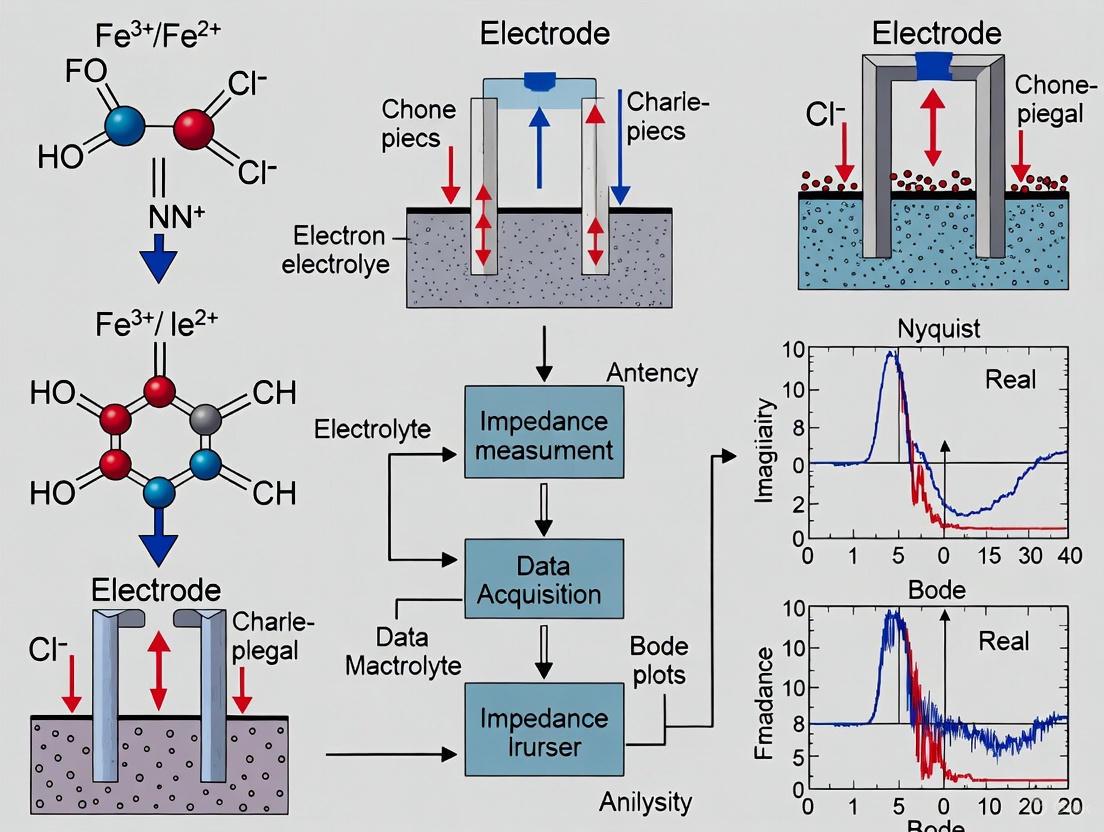
The introduction of a redox-active species, or a redox probe, is what enables the Faradaic process. Commonly used probes include ferro/ferricyanide ([Fe(CN)6]3−/4−) and hexaammineruthenium ([Ru(NH3)6]3+/2+). When the target analyte interacts with the sensor surface—be it through binding, blocking, or altering the interface—it impedes the redox probe's access or electron transfer kinetics. This obstruction causes a measurable increase in the Rct value, providing the quantitative foundation for sensing [11] [10]. The following diagram illustrates the core signaling mechanism of a Faradaic EIS biosensor.

The electrical characteristics of the electrode-electrolyte interface in a Faradaic EIS system are accurately modeled by an equivalent circuit. The most common model is the Randles-Ershler equivalent circuit, which includes the following components [9] [11] [10]:

• Rs: The solution resistance.
• Cdl: The double-layer capacitance.
• Rct: The charge-transfer resistance.
• W: The Warburg impedance, representing diffusion.

In this circuit, the Rct is the parameter most directly influenced by surface binding events and is therefore the primary correlate for analyte concentration.

Experimental Protocols

Protocol 1: Electrode Modification and Sensor Fabrication (Exemplified for a Metallic Nanoparticle-Based Sensor)

This protocol outlines the fabrication of a glassy carbon electrode (GCE) modified with oxidized multiwalled carbon nanotubes (MWCNTs) and gold nanoparticles (AuNPs) for the detection of a thiol-containing drug, adapted from a published sensor for Mesna [11].

• Aim: To create a high-sensitivity impedimetric sensor with enhanced surface area and electrocatalytic activity.

• Materials:

  • Glassy Carbon Electrode (GCE): Serves as the conductive base transducer.
  • Oxidized MWCNTs: Provide a high surface area and facilitate electron transfer.
  • Chloroauric Acid (HAuCl4): Precursor for gold nanoparticle synthesis.
  • Potassium Ferricyanide/Ferrocyanide ([Fe(CN)6]3−/4−): Redox probe solution.
  • Phosphate Buffered Saline (PBS) or KCl: Electrolyte solution.
  • Target Analyte Standard: e.g., Mesna drug solution.

• Procedure:

  • Electrode Polishing: Polish the bare GCE sequentially with alumina slurries (e.g., 1.0, 0.3, and 0.05 µm) on a microcloth pad. Rinse thoroughly with deionized water after each polish.
  • MWCNT Dispersion: Prepare a homogeneous dispersion of oxidized MWCNTs (e.g., 1 mg/mL) in a suitable solvent like dimethylformamide (DMF) using ultrasonication.
  • MWCNT Modification: Drop-cast a precise volume (e.g., 5 µL) of the MWCNT dispersion onto the polished surface of the GCE and allow it to dry under ambient conditions to form the MWCNTs/GCE.
  • AuNPs Electrodeposition: Immerse the MWCNTs/GCE in an aqueous solution of HAuCl4 (e.g., 0.5 mM in 0.1 M KNO3). Perform electrodeposition by cycling the potential (e.g., between -0.2 and +1.0 V vs. Ag/AgCl for 10 cycles) to form AuNPs/MWCNTs/GCE.
  • Sensor Characterization: Use Cyclic Voltammetry (CV) and EIS in a solution containing your chosen redox probe (e.g., 5 mM [Fe(CN)6]3−/4− in 0.1 M KCl) to confirm the successful modification. A significant decrease in Rct compared to the bare GCE indicates enhanced electron transfer kinetics.

Protocol 2: EIS Measurement and Analytical Calibration

This protocol describes the standard procedure for acquiring impedimetric data and constructing a calibration curve for quantitative analysis.

• Aim: To measure the charge transfer resistance (Rct) and establish a correlation with analyte concentration.

• Materials:

  • Fabricated sensor (e.g., from Protocol 1).
  • Potentiostat with EIS capability.
  • Electrochemical cell with Ag/AgCl reference and Pt counter electrodes.
  • Redox probe in supporting electrolyte (e.g., 5 mM [Fe(CN)6]3−/4− in 0.1 M KCl).
  • Standard solutions of the target analyte at known concentrations.

• Procedure:

  • Baseline EIS Measurement: Place the modified sensor in the electrochemical cell containing the redox probe/electrolyte solution. Record the EIS spectrum at the formal potential of the redox probe (e.g., +0.22 V vs. Ag/AgCl for [Fe(CN)6]3−/4−). Typical parameters: frequency range from 0.01 Hz to 100 kHz, AC amplitude of 10 mV. This measurement provides the baseline Rct (Rct,0).
  • Analyte Incubation: Incubate the sensor with a standard solution of the target analyte for a fixed duration under controlled conditions (e.g., 15 minutes at room temperature).
  • Post-Incubation EIS Measurement: Rinse the sensor gently with the supporting electrolyte to remove unbound molecules. Re-immerse it in the fresh redox probe/electrolyte solution and record a new EIS spectrum under identical conditions. This provides Rct after analyte binding (Rct,A).
  • Data Fitting: Fit the obtained Nyquist plots using the Randles equivalent circuit model to extract precise Rct values.
  • Calibration Curve: Repeat steps 1-4 for at least five different standard concentrations of the analyte. Plot the relative change in charge transfer resistance, often expressed as (Rct,A - Rct,0)/Rct,0 or simply Rct,A, against the logarithm of the analyte concentration. Perform linear or non-linear regression to establish the quantitative relationship.

The workflow below summarizes this process from sensor preparation to data analysis.

Data Presentation & Analysis

Performance Comparison of Common Redox Probes

The choice of redox probe is critical and depends on the sensor surface and the intended application. The table below summarizes the key characteristics of two widely used probes.

Table 1: Comparison of Common Redox Probes in Faradaic EIS

Property	[Fe(CN)6]3−/4−	[Ru(NH3)6]3+/2+
Electron Transfer Kinetics	Quasi-reversible, surface-sensitive [12]	Near-ideal, outer-sphere [12]
Cost	Inexpensive [12]	High cost [12]
Key Advantage	Low cost, widely adopted	Insensitive to surface microstructure and moderate roughness [12]
Key Limitation	Sensitive to surface chemistry and surface states on carbon electrodes; kinetics can be influenced by surface functional groups [12]	High cost can be prohibitive for some laboratories [12]
Ideal Use Case	Preliminary characterization on metal electrodes; systems where cost is a primary driver	Accurate assessment of true electron transfer rates; studies on carbon-based or rough electrodes [12]

Exemplary Analytical Performance

The following table presents performance data from real research to illustrate the sensitivity and dynamic range achievable with optimized Faradaic EIS sensors.

Table 2: Exemplary Analytical Performance of Reported Faradaic EIS Sensors

Analyte	Sensor Platform	Redox Probe	Linear Range	Detection Limit	Application
Mesna (anti-cancer drug)	AuNPs/MWCNTs /GCE [11]	[Fe(CN)6]3−/4−	0.06 nM - 1.0 nM & 1.0 nM - 130.0 µM [11]	0.02 nM [11]	Serum & urine samples [11]
Alpha-synuclein Oligomers (Parkinson's biomarker)	Aptamer/Au electrode [13]	[Fe(CN)6]3−/4−	Not specified	Good sensitivity and selectivity reported [13]	Buffer solution [13]

The Scientist's Toolkit: Essential Research Reagents & Materials

Table 3: Key Reagents and Materials for Faradaic EIS Sensing

Item	Function/Description	Example
Redox Probe	Generates the Faradaic current; its electron transfer is modulated by the analyte.	Potassium ferricyanide/ferrocyanide ( [Fe(CN)6]3−/4− ) [11] [14]
Supporting Electrolyte	Carries ionic current, minimizes solution resistance (Rs), and controls ionic strength.	Potassium Chloride (KCl), Phosphate Buffered Saline (PBS) [15] [14]
Electrode Modifiers	Enhance surface area, improve electron transfer kinetics, and provide sites for biorecognition.	MWCNTs, Gold Nanoparticles (AuNPs), Graphene [11]
Biorecognition Element	Imparts selectivity by specifically binding the target analyte.	Antibodies, Aptamers, Enzymes, Molecularly Imprinted Polymers (MIPs) [16] [13]
Repinotan hydrochloride	Repinotan Hydrochloride|5-HT1A Receptor Agonist	Repinotan hydrochloride is a potent, selective 5-HT1A receptor agonist for neuroscience research. For Research Use Only. Not for human or veterinary diagnostic or therapeutic use.
3-Acetyl-5-bromopyridine	3-Acetyl-5-bromopyridine | High Purity | For RUO	3-Acetyl-5-bromopyridine: A versatile brominated & acetylated pyridine scaffold for pharmaceutical & materials research. For Research Use Only. Not for human use.

Troubleshooting and Best Practices

• Probe and Electrolyte Optimization: The concentration of the redox probe and the ionic strength of the background electrolyte significantly impact the Nyquist plot. Increasing ionic strength can shift the RC semicircle to higher frequencies. Optimization is required to achieve a clear, measurable semicircle in the accessible frequency range [15].
• Stability of Rct Baseline: Ensure the Rct of the sensor is stable in the pure redox solution before analyte introduction. Drifting baselines indicate an unstable modification layer or electrode fouling.
• Control Experiments: Always perform control experiments to confirm that the observed Rct change is due to specific analyte binding and not non-specific adsorption or changes in solution conditions.
• Circuit Model Validation: Use the Kramers-Kronig transforms to check the stability and linearity of the system. Ensure the chosen equivalent circuit model provides a good fit to the experimental data across the entire frequency range [9].
• Surface Regeneration: For reusable sensors, develop a gentle and effective regeneration protocol (e.g., a mild pH wash) that removes the bound analyte without damaging the biorecognition layer on the sensor surface.

The Randles circuit is a fundamental equivalent electrical model used to interpret the impedance response of electrochemical interfaces, particularly in faradaic processes central to redox sensing and biosensing research [17]. It provides a physical model for describing the processes at an electrode-solution interface where a dissolved electroactive species undergoes a reduction or oxidation reaction [18]. For researchers developing electrochemical sensors for drug analysis or diagnostic applications, mastering the Randles circuit is essential for extracting meaningful physicochemical parameters from impedance spectra, enabling the quantification of interfacial properties, reaction kinetics, and mass transport effects that define sensor performance.

This application note deconstructs the circuit's core components within the context of EIS-based redox sensing, providing detailed protocols for experimental measurement, data fitting, and interpretation relevant to biomedical and pharmaceutical research.

Circuit Components and Their Physical Meaning

The Randles circuit models an electrochemical cell using a combination of passive electrical elements, each representing a distinct physical process at the electrode-solution interface [17]. A thorough understanding of each component is crucial for diagnosing sensor behavior and optimizing its design.

Table 1: Core Components of the Randles Circuit

Component	Symbol	Physical Origin	Impedance Formula
Solution Resistance	RΩ	Ionic resistance of the electrolyte solution between working and reference electrodes [17]	Z = RΩ [2]
Double Layer Capacitance	Cdl	Charge separation at the electrode-electrolyte interface, forming the electrochemical double-layer [3] [18]	Z = 1/(jωCdl) [2]
Charge Transfer Resistance	Rct	Resistance to electron transfer across the interface during a faradaic reaction [18] [17]	Z = Rct [2]
Warburg Impedance	W	Resistance due to diffusion of electroactive species from the bulk solution to the electrode surface [17] [19]	ZW = AW/√ω + AW/(j√ω) [17]

The Complete Model and Its Spectrum

These components are combined such that the solution resistance, R_Ω, is in series with a parallel combination of the double-layer capacitance, C_dl, and a series combination of the charge-transfer resistance, R_ct, and the Warburg impedance, W [17]. The resulting Nyquist plot provides a distinctive fingerprint of the electrochemical system.

Figure 1: Randles circuit diagram showing component relationships. Rct and W are in series, and this series combination is in parallel with Cdl. The entire parallel network is in series with RΩ.

Experimental Protocol for EIS Measurement

This protocol outlines the steps for acquiring high-quality impedance spectra of a redox couple in solution, suitable for fitting to the Randles circuit model.

Research Reagent Solutions

Table 2: Essential Materials and Reagents

Item	Function	Example Specification
Potentiostat with EIS Capability	Applies potential and measures current response.	Must include a frequency response analyzer (FRA); capable of 10 mHz to 100 kHz [18].
Three-Electrode Cell	Provides controlled electrochemical environment.	Cell vial, working electrode (e.g., 2 mm gold disk), counter electrode (platinum wire), reference electrode (Ag/AgCl) [3].
Redox Probe	Provides the faradaic reaction for sensing.	5 mM Potassium Ferricyanide (K3[Fe(CN)6]) in supporting electrolyte [19].
Supporting Electrolyte	Carries current and minimizes migration.	1 M Potassium Chloride (KCl) or other inert salt.
Solvent	Dissolves redox probe and electrolyte.	Deionized Water, PBS buffer, or other appropriate solvent.

Step-by-Step Procedure

• Cell Setup: Clean the working electrode according to standard procedures (e.g., polishing for solid electrodes). Place the working, reference, and counter electrodes into the cell containing your redox probe solution in a supporting electrolyte [3].
• Establish DC Potential: Apply the DC potential (E_DC) around the formal potential of the redox couple. For a reversible couple like Fe(CN)₆^3-/4-, this is typically +0.22 V vs. Ag/AgCl. Allow the current to stabilize, indicating a steady-state condition [20].
• Configure EIS Parameters: Set the AC excitation parameters on the potentiostat.
  • Frequency Range: Typically from 100 kHz to 100 mHz (or 10 mHz for full diffusion control) [18].
  • AC Amplitude: A small, 10 mV sinusoidal perturbation is standard to ensure the system response is pseudo-linear [18] [2].
  • Points per Decade: 5 to 10 points per frequency decade for sufficient spectral definition.
• Run EIS Measurement: Initiate the frequency sweep. The instrument will apply the sine wave at each frequency, measure the current response's amplitude and phase shift, and calculate the impedance [3].
• Data Quality Validation: Use instrument software to check quality indicators like Total Harmonic Distortion (THD) to verify linearity and Non-Stationary Distortion (NSD) to ensure system stability during measurement. A THD below 5% is generally acceptable [20].

Data Interpretation and Analysis

The acquired EIS data is most commonly visualized using a Nyquist plot, which provides a characteristic shape for the Randles circuit.

Visualizing the Impedance Spectrum

Figure 2: Characteristic Nyquist plot of a Randles circuit, showing the high-frequency semicircle and low-frequency Warburg line.

Extracting Circuit Parameters

• Step 1: Estimate R_Ω. Identify the left-most intercept of the impedance spectrum with the real (Z') axis. This value represents the uncompensated solution resistance, R_Ω [21].
• Step 2: Estimate R_ct. Determine the diameter of the semicircular portion of the spectrum. The difference between the real-axis value at the low-frequency end of the semicircle and R_Ω gives the charge transfer resistance, R_ct [21].
• Step 3: Calculate C_dl. The characteristic frequency (f_max) at the top of the semicircle (where -Z'' is maximum) is related to the time constant of the interface: C_dl = 1 / (2Ï€f_maxR_ct) [21].
• Step 4: Identify Diffusion Control. At lower frequencies, a straight line at a 45° angle indicates Warburg impedance, signifying that the overall reaction rate is limited by the diffusion of the electroactive species [17] [19].

Advanced Analysis: Equivalent Circuit Fitting

For precise quantification, experimental data should be fitted using EIS software.

• Select the Randles circuit model as the fitting function.
• Use the estimated values from the visual inspection as initial guesses for the fitting algorithm.
• Run a complex non-linear least squares (CNLS) fitting procedure to obtain refined values for R_Ω, C_dl, R_ct, and the Warburg coefficient, A_W [17].
• Validate the fit by overlaying the simulated spectrum from the fitted parameters onto the experimental data.

Application in Redox Sensing Research

The parameters derived from the Randles circuit are powerful indicators of interfacial properties and reaction kinetics, directly applicable to biosensor development.

• Probing Surface Modification: Successful immobilization of a capture probe (e.g., an antibody or DNA strand) on an electrode surface creates an insulating layer. This hinders electron transfer of a solution-based redox probe ([Fe(CN)₆]^3-/4-), resulting in a measurable increase in R_ct. This increase can be used to confirm and quantify functionalization [18].
• Detecting Binding Events: The specific binding of a target analyte (e.g., a protein or drug molecule) to the immobilized capture layer further impedes access to the redox probe. This is observed as a further increase in R_ct, enabling the quantitative detection of the analyte. The change in R_ct (ΔR_ct) can be correlated with analyte concentration.
• Diagnosing Sensor Performance: A significant Warburg impedance (45° line) at typical measurement frequencies suggests the sensor response is diffusion-limited rather than reaction-limited. This may indicate a need for optimization, such as reducing the measurement frequency, enhancing surface area, or improving stirring, to ensure the sensor's response is governed by the binding event itself.

The Randles circuit transforms a complex electrochemical interface into a quantifiable model. By systematically deconstructing its components and following rigorous experimental and analytical protocols, researchers can effectively design, characterize, and optimize sensitive EIS-based redox sensors for drug development and diagnostic applications.

Electrochemical Impedance Spectroscopy (EIS) is a powerful analytical technique that has revolutionized the characterization of electrochemical systems, particularly in the field of redox sensing for biomedical and pharmaceutical applications. As a non-destructive, label-free method, EIS provides kinetic and mechanistic data by probing the frequency-dependent impedance of an electrochemical interface [22]. In redox sensing, this enables the detailed study of electron transfer processes and mass transport phenomena that occur during biorecognition events, such as antibody-antigen interactions, substrate-enzyme reactions, or whole cell capturing [23]. The technique operates on the principle of applying a small-amplitude sinusoidal potential (typically 1-10 mV) to an electrochemical cell and measuring the current response across a wide frequency range (from μHz to MHz) [2] [22]. The resulting data, when visualized through Nyquist and Bode plots, offers a wealth of information about the system under investigation, allowing researchers to deconvolve complex processes into discrete elements with different time constants [22].

For researchers in drug development, EIS presents particular advantages for monitoring binding events in real-time without the need for fluorescent or radioactive labels, making it ideal for studying delicate biological interactions in their native states. The sensitivity of EIS to surface modifications enables the detection of low-abundance biomarkers when proper optimization is performed [15]. This application note provides a comprehensive guide to interpreting the primary visualization tools in EIS—Nyquist and Bode plots—with a specific focus on extracting meaningful information about electron transfer and diffusion processes critical to redox sensing applications.

Theoretical Background

Fundamental Principles of EIS

In EIS, a sinusoidal potential excitation signal is applied to an electrochemical system, and the resulting current response is measured. For a linear, time-invariant system, the response will be a sinusoid at the same frequency but shifted in phase [2]. The excitation potential is described by the equation:

[ Et = E0 \cdot \sin(\omega t) ]

where ( Et ) is the potential at time ( t ), ( E0 ) is the amplitude of the signal, and ( \omega ) is the radial frequency [23]. The relationship between radial frequency and applied frequency ( f ) is given by ( \omega = 2 \pi f ) [23].

The current response is described by:

[ It = I0 \cdot \sin(\omega t + \Phi) ]

where ( I_0 ) is the amplitude of the current signal, and ( \Phi ) is the phase shift between potential and current [23] [2].

Impedance (( Z )) is then defined as the complex ratio of potential to current:

[ Z = \frac{E}{I} = Z_0 \cdot (\cos\Phi + j\sin\Phi) ]

where ( Z ) is expressed in terms of magnitude ( Z_0 ) and phase shift ( \Phi ) [23] [2]. This complex impedance can be separated into real (( Z' )) and imaginary (( Z'' )) components:

[ Z = Z' + jZ'' ]

where ( Z' = |Z|\cos\Phi ) and ( Z'' = |Z|\sin\Phi ) [20].

Critical Requirements for Valid EIS Measurements

Two fundamental requirements must be met for reliable EIS measurements: linearity and stationarity. Electrochemical systems are inherently non-linear, but linearity can be approximated by using sufficiently small excitation amplitudes (typically 1-10 mV) [2] [20]. This ensures the system response is pseudo-linear within the small perturbation region around the operating point. Stationarity requires that the system remains stable throughout the measurement duration, which can range from minutes to hours depending on the frequency range scanned [2] [20]. Non-stationary distortion (NSD) and total harmonic distortion (THD) indicators can be used to validate these conditions, with THD values below 5% generally indicating acceptable linearity [20].

Data Representation and Interpretation

Nyquist Plots

The Nyquist plot represents one of the most common forms of EIS data visualization in electrochemical research. In this representation, the negative imaginary impedance (( -Z'' )) is plotted against the real part of the impedance (( Z' )) across all measured frequencies [21] [23]. Each point on the Nyquist plot corresponds to the impedance at a specific frequency, though the frequency values are not explicitly shown along the curve [2]. Conventionally, high-frequency data appears on the left side of the plot, while low-frequency data appears on the right [23] [2]. It is crucial to use an orthonormal scale (1:1 aspect ratio) for Nyquist plots to prevent visual distortion and misinterpretation of the data [20].

In a typical Nyquist plot of a Faradaic system, several distinct regions provide information about different processes:

• The high-frequency intercept with the x-axis represents the solution resistance (( R_s ))
• A semicircular region at higher frequencies corresponds to the charge transfer process
• A linear region at lower frequencies (at a 45° angle for an ideal system) represents mass transport limitations [23]

The diameter of the semicircle in the Nyquist plot equals the charge transfer resistance (( R_{ct} )), a key parameter in redox sensing as it characterizes the kinetics of electron transfer across the electrode-electrolyte interface [21] [24].

Bode Plots

The Bode plot provides an alternative representation of EIS data that explicitly shows frequency information. A Bode plot consists of two separate graphs: (1) the logarithm of impedance magnitude (( \log |Z| )) versus the logarithm of frequency (( \log f )), and (2) the phase shift (( \Phi )) versus ( \log f ) [21] [23]. This representation offers several advantages for certain applications, as all impedance information is clearly visible, and individual circuit components can be more easily understood compared to Nyquist plots [21].

In redox sensing applications, Bode plots are particularly valuable for:

• Identifying time constants of different processes through phase angle peaks
• Evaluating the capacitive behavior of the electrochemical double layer
• Assessing system stability across frequencies
• Determining the frequency range where diffusion processes dominate [23]

The Bode plot often shows a plateau in impedance magnitude at high frequencies (representing solution resistance), a sloping region at intermediate frequencies (related to charge transfer processes), and another plateau or different slope at low frequencies (indicating mass transport control) [3]. Simultaneously, the phase angle plot typically shows characteristic peaks that correspond to different time constants in the system.

Comparative Analysis of Plot Types

Table 1: Comparison of Nyquist and Bode Plots for EIS Data Representation

Feature	Nyquist Plot	Bode Plot
Axes	-Z'' vs Z' (complex plane)	log|Z| vs log(f) and Φ vs log(f)
Frequency Information	Implicit (not directly visible)	Explicit (frequency is the x-axis)
Primary Strengths	Sensitive to small changes; popular in electrochemistry; easy parameter estimation for simple circuits	Clear visualization of frequency dependence; easier to identify individual components
Common Applications	Quick assessment of charge transfer resistance; corrosion studies; battery analysis	Capacitive system analysis; identifying time constants; system stability assessment
Interpretation Challenges	Frequency values not displayed; complex to understand for beginners	Requires reading two graphs simultaneously; less intuitive for complex circuits

Equivalent Circuit Modeling

The Randles Circuit

The Randles circuit represents the most fundamental equivalent circuit model for describing a simple electrochemical system with a single electron transfer reaction, making it highly relevant to redox sensing applications [21] [22]. This circuit includes:

• Solution resistance (( R_s )): representing the ionic resistance of the electrolyte
• Double layer capacitance (( C_{dl} )): representing the capacitor formed at the electrode-electrolyte interface
• Charge transfer resistance (( R_{ct} )): representing the resistance to electron transfer across the interface
• Warburg impedance (( W )): representing mass transport limitations [21] [23]

In the Nyquist plot, the Randles circuit produces a characteristic semicircle at higher frequencies (from the parallel combination of ( C{dl} ) and ( R{ct} )) followed by a 45° linear region at lower frequencies (from the Warburg element) [21]. In Bode representation, the Randles circuit shows a phase angle peak corresponding to the time constant of the charge transfer process.

Circuit Elements and Their Physical Meaning

Table 2: Equivalent Circuit Elements and Their Physical Significance in Redox Sensing

Circuit Element	Impedance Equation	Physical Meaning	Visual Representation in Plots
Resistor (R)	( Z = R )	Solution resistance (Rₛ) or charge transfer resistance (R_ct)	Nyquist: Point on x-axis Bode: Horizontal line for |Z|, 0° phase
Capacitor (C)	( Z = 1/(j\omega C) )	Double layer capacitance (C_dl)	Nyquist: Straight vertical line Bode: -1 slope for |Z|, -90° phase
Warburg (W)	( Z = \sigma\omega^{-1/2}(1-j) )	Semi-infinite diffusion	Nyquist: 45° line Bode: -0.5 slope for |Z|, 45° phase
Constant Phase Element (CPE)	( Z = 1/[Q(j\omega)^n] )	Non-ideal capacitance (surface heterogeneity)	Nyquist: Depressed semicircle Bode: Variable phase angle

Experimental Protocols

Protocol for EIS Measurement in Redox Sensing

This protocol outlines the standardized procedure for conducting EIS measurements in redox sensing applications, adapted from established methodologies with specific considerations for pharmaceutical and biosensing applications [24].

Electrode Preparation and System Setup

• Working Electrode Preparation: Polish a 1-3 mm diameter platinum or gold working electrode for 30 seconds using a polishing cloth moistened with alumina slurry (0.05 μm). Rub the flat surface of the disc electrode with moderate pressure to ensure a mirror-like finish [24].

• Electrode Cleaning: Rinse the electrode thoroughly with distilled water three times to remove all alumina particles, followed by rinsing with the solvent to be used in the experiment (e.g., dichloromethane for organic systems or purified water for aqueous systems) [24].

• Counter Electrode Preparation: Anneal a platinum wire counter electrode in a butane burner flame for less than 1 second until it begins reddening, then quickly remove to avoid melting. Ensure the counter electrode surface area is significantly larger than the working electrode to minimize its contribution to the total impedance [24].

• Reference Electrode Preparation: For non-aqueous systems, prepare a pseudo-reference electrode (e.g., silver wire) by annealing in a butane burner flame using the same method as the counter electrode. For aqueous systems, use a standard reference electrode such as Ag/AgCl [24].

• Cell Assembly: Place all three electrodes into the electrochemical cell containing the analyte solution, ensuring they do not contact each other. Connect to the corresponding potentiostat cables marked WE (working electrode), CE (counter electrode), and RE (reference electrode) [24].

• Solution Deaeration: Insert a gas delivery tube connected to an inert gas supply (argon or nitrogen) and bubble through the solution for 20 minutes to remove dissolved oxygen. Maintain a slight positive pressure of inert gas during measurements when oxygen sensitivity is a concern [24].

Cyclic Voltammetry Characterization

• Initial CV Setup: Program the potentiostat for cyclic voltammetry with an initial potential of 0.0 V, switching potentials appropriate for the redox system under study (typically ±2.0 V for unknown systems), and a scan rate of 100 mV/s [24].

• Preliminary CV: Run the cyclic voltammetry to identify the approximate formal potential (E⁰) of the redox couple. Note the potential values at the maxima of the anodic and cathodic peaks and calculate their average to estimate E⁰ [24].

• Internal Standard Addition: Add a small amount (approximately 10 mg) of ferrocene as an internal standard for non-aqueous systems. Deaerate for an additional 5 minutes to ensure mixing and complete dissolution [24].

• Reference CV: Run an additional CV scan focusing on the region around the ferrocene/ferrocenium redox couple (typically -1.0 V to +1.0 V) to accurately determine the reference potential [24].

• Formal Potential Determination: Calculate the formal potential of your target redox couple relative to the ferrocene/ferrocenium couple (Fc/Fc⁺), which is typically used as an internal standard with E⁰ defined as 0 V [24].

EIS Measurement Procedure

• Parameter Setup: Configure the potentiostat for potentiostatic EIS measurement with the following typical parameters [24]:

  • DC potential: Set to the formal potential (E⁰) of the redox couple determined from CV
  • AC amplitude: 10 mV (ensure linearity conditions)
  • Frequency range: 10 kHz to 100 Hz (preliminary) or 100 kHz to 0.1 Hz (comprehensive)
  • Points per decade: 10-20 (logarithmically spaced)
  • Wait time between measurements: 5 seconds (to ensure stability)

• Preliminary Spectrum: Run an initial impedance spectrum to verify system behavior and signal quality.

• Potential Mapping: For detailed kinetic analysis, program an automated potential staircase measurement with the following parameters [24]:

  • Potential range: E⁰ ± 0.2 V
  • Potential increment: 0.01 V
  • Number of spectra: 41 (for ±0.2 V range)
  • Other parameters as in step 1

• Data Collection: Initiate the automated EIS measurement series. The total measurement time will depend on the frequency range and points per decade but typically requires 2-3 minutes per spectrum [24].

• Quality Validation: Monitor THD and NSD indicators during measurement to ensure data quality. THD should remain below 5% to verify linearity, and NSD should be minimal to confirm stationarity [20].

The Scientist's Toolkit: Essential Research Reagents and Materials

Table 3: Essential Research Reagents and Materials for EIS in Redox Sensing

Reagent/Material	Specification	Function in Experiment
Supporting Electrolyte	0.1 M Buâ‚„NBFâ‚„ (for organic systems) or 0.1 M KCl/PBS (for aqueous systems)	Provides ionic conductivity; minimizes solution resistance
Redox Probe	1-5 mM Ferro/ferricyanide ([Fe(CN)₆]³⁻/⁴⁻) or [Ru(bpy)₃]²⁺	Generates Faradaic current; enhances sensitivity to surface changes
Working Electrode	Pt or Au disk (1-3 mm diameter)	Platform for electron transfer; surface for biorecognition element immobilization
Reference Electrode	Ag/AgCl (aqueous) or Ag wire (non-aqueous)	Provides stable reference potential for accurate potential control
Counter Electrode	Pt wire (large surface area)	Completes electrical circuit; prevents current limitation
Polishing Materials	Alumina slurry (0.05 μm) and polishing cloth	Ensizes reproducible electrode surface; removes contaminants
Solvent	Dichloromethane (organic) or buffer (aqueous)	Dissolves analyte and electrolyte; determines double layer structure
5,7-Dihydroxy-4-Methylphthalide	5,7-Dihydroxy-4-methylphthalide|CAS 27979-57-3	5,7-Dihydroxy-4-methylphthalide is a key precursor for mycophenolic acid biosynthesis. This product is for Research Use Only (RUO). Not for human use.
6-Aldehydoisoophiopogonone A	6-Aldehydo-isoophiopogonone A|CAS 112500-90-0|RUO

Data Analysis and Interpretation

Analyzing Nyquist Plots for Electron Transfer and Diffusion

In redox sensing applications, the analysis of Nyquist plots focuses on extracting parameters related to electron transfer kinetics and mass transport limitations. The charge transfer resistance (( R_{ct} )) is obtained from the diameter of the semicircle in the high-frequency region and is inversely proportional to the standard rate constant of the electron transfer reaction [24]:

[ R_{ct} = \frac{RT}{nF} \cdot \frac{1}{k^0 \cdot A \cdot c} ]

where ( R ) is the gas constant, ( T ) is temperature, ( n ) is the number of electrons transferred, ( F ) is Faraday's constant, ( k^0 ) is the standard rate constant, ( A ) is the electrode area, and ( c ) is the concentration of the redox species [24].

For diffusion-controlled processes, the low-frequency region of the Nyquist plot shows a Warburg impedance, which appears as a straight line with a 45° slope for semi-infinite linear diffusion. The point where the semicircle transitions to the Warburg line provides information about the characteristic frequency of the diffusion process, from which the diffusion coefficient can be calculated [23].

In the context of redox sensing, changes in ( R{ct} ) are particularly important as they often indicate binding events or surface modifications that affect electron transfer kinetics. For example, when a target molecule binds to a capture probe immobilized on the electrode surface, it typically increases ( R{ct} ) by creating an additional barrier to electron transfer, enabling quantitative detection of the target analyte [15].

Extracting Parameters from Bode Plots

Bode plots provide complementary information that is particularly valuable for identifying processes with different time constants. The frequency at which the phase angle reaches a maximum (( f_{max} )) is related to the time constant (( \tau )) of the corresponding process [22]:

[ \tau = \frac{1}{2\pi f{max}} = R{ct} \cdot C_{dl} ]

This relationship allows researchers to deconvolve processes with similar resistances but different time constants, which is common in complex biological systems where multiple processes occur simultaneously.

The magnitude plot also provides information about the dominant process at different frequency regimes:

• At high frequencies: ( |Z| ) approaches ( R_s ) (solution resistance)
• At intermediate frequencies: The slope of ( \log |Z| ) vs ( \log f ) indicates the dominant process (-1 for capacitive, -0.5 for diffusion)
• At low frequencies: ( |Z| ) approaches ( Rs + R{ct} ) for kinetically controlled systems or shows continued decrease for diffusion-controlled systems

Equivalent Circuit Modeling and Validation

After collecting EIS data, researchers typically fit the results to an equivalent circuit model to extract quantitative parameters. The following protocol outlines this process:

• Circuit Selection: Start with the simplest plausible circuit (e.g., a modified Randles circuit) and progressively increase complexity if needed [24].

• Initial Parameter Estimation: Estimate initial values for circuit elements based on the EIS plot:

  • ( R_s ): High-frequency intercept on Nyquist plot
  • ( R_{ct} ): Diameter of the semicircle
  • ( C{dl} ): Estimate from ( C{dl} = 1/(2\pi f{max} R{ct}) ) where ( f_{max} ) is the frequency at the top of the semicircle

• Non-linear Least Squares Fitting: Use specialized software (e.g., ZView, EC-Lab, or similar) to perform non-linear least squares fitting of the model to the experimental data [24].

• Goodness-of-Fit Evaluation: Assess the quality of the fit using parameters such as χ² value (should be <10⁻³ for a good fit) and visual inspection of residuals [24].

• Model Validation: Apply the Kramers-Kronig relations to test the validity of the data, ensuring compliance with linearity, causality, and stability conditions [22].

• Parameter Error Assessment: Check the relative errors of fitted parameters. If any parameter has an error exceeding 100%, consider simplifying the model as that parameter may not be necessary [24].

Advanced Applications in Redox Sensing

The integration of EIS with redox sensing has enabled significant advances in biomedical research and drug development. Recent studies have demonstrated the utility of EIS in detecting various analytes including pathogens, DNA biomarkers, cancer-associated proteins, and emerging chemical contaminants [23] [15]. The exceptional sensitivity of EIS stems from its ability to detect minor changes in interfacial properties resulting from biorecognition events.

Nanomaterials have played a crucial role in enhancing EIS-based biosensors by providing catalytic activity, facilitating sensing element immobilization, promoting faster electron transfer, and increasing reliability [23]. For example, the incorporation of nanoparticles, nanotubes, and nanocomposites has been shown to significantly improve the analytical performance of impedimetric biosensors [23].

Recent research has also focused on optimizing electrolyte and redox probe systems to enhance sensitivity. Studies have shown that by carefully controlling the ionic strength of the background electrolyte and the concentration of the redox probe, researchers can tune the frequency response of the system to maximize sensitivity to specific binding events [15]. This optimization has enabled the transition from expensive laboratory impedance analyzers to more affordable portable systems, making EIS-based sensing more accessible for point-of-care applications [15].

Troubleshooting and Best Practices

Common Issues and Solutions

• Non-Linear Response: If THD values exceed 5%, reduce the AC amplitude (while maintaining adequate signal-to-noise ratio) or verify that the DC potential is correctly set [20].

• Non-Stationary Behavior: If NSD indicates time-variance, ensure system stability by controlling temperature, minimizing evaporation, and verifying that electrochemical processes are at steady-state before measurement [20].

• Noisy Low-Frequency Data: Increase the number of measurement cycles per frequency or apply digital filtering to improve signal quality at low frequencies where measurement time is longest.

• Poor Fitting Results: Verify the appropriateness of the equivalent circuit model, check for unaccounted-for processes, and ensure data quality meets Kramers-Kronig criteria [22] [24].

• Irreproducible Results: Standardize electrode preparation procedures, ensure consistent surface cleaning, and verify electrolyte composition and degassing protocols [24].

Optimization Strategies for Redox Sensing

• Redox Probe Selection: Choose redox probes with formal potentials that do not interfere with the biological system under study. Common choices include ferro/ferricyanide for aqueous systems and ferrocene derivatives for organic systems [15].

• Surface Modification: Optimize the density of capture probes on the electrode surface to balance accessibility for target binding with sufficient spacing to minimize steric hindrance.

• Frequency Range Selection: Focus on the frequency range that is most sensitive to the process of interest. For binding-induced changes in charge transfer, the frequency around the phase maximum typically provides the greatest sensitivity.

• Signal Normalization: Always normalize impedance parameters to electrode surface area when comparing between different electrodes or experiments.

Through proper implementation of the protocols and interpretation methods outlined in this application note, researchers can leverage the full power of EIS for advancing redox sensing applications in drug development and biomedical research.

Why Linearity and Stationarity are Non-Negotiable for Reliable EIS Measurements

In the field of electrochemical impedance spectroscopy (EIS) for redox sensing, the reliability of data interpretation hinges on fulfilling two fundamental system requirements: linearity and stationarity. These conditions are not merely advantageous but are absolute prerequisites for obtaining physically meaningful results that can accurately describe electrochemical interfaces and processes. EIS functions by applying a small sinusoidal perturbation to an electrochemical system and analyzing the resulting response [20]. The technique is founded on the assumption that the system under study behaves as a Linear Time-Invariant (LTI) system for the duration of the measurement [20]. Violations of either linearity or stationarity introduce significant distortions, rendering the resulting impedance data invalid and leading to erroneous conclusions in redox sensing research. This application note details the theoretical and practical aspects of these requirements, providing validated protocols to ensure data integrity.

Theoretical Underpinnings

The Principle of Linearity

Electrochemical systems are inherently non-linear, as described by fundamental relationships such as the Butler-Volmer equation for charge-transfer kinetics. The principle of linearity stipulates that the response of the system (current output) must be directly proportional to the perturbation (voltage input) [20]. In practice, this condition is achieved not by altering the system's intrinsic properties, but by restricting the measurement to a sufficiently small amplitude perturbation. As shown in Figure 1, a small enough excitation signal ensures that the system's response approximates the tangent of its steady-state current-potential curve, creating an effectively linear region around the operating point (DC bias) [20]. This small-signal approximation is critical for applying the fundamental laws of impedance.

The Principle of Stationarity

The principle of stationarity, or time-invariance, requires that the properties of the electrochemical system being measured remain constant throughout the entire duration of the impedance frequency sweep [20]. Any significant drift in parameters—such as surface concentration of redox species, electrode active area due to corrosion or deposition, or temperature—violates this condition. A system must first be in a steady-state (not in a transient phase) before an EIS measurement begins, and must maintain that state during the measurement. This is particularly challenging in systems involving dynamic interfacial changes, such as the cycling of lithium metal electrodes, where operando EIS requires specialized approaches to deconvolute these changes [25].

Consequences of Violating LTI Conditions

Effects of Non-Linearity

When the applied perturbation amplitude is too large, the system operates outside the linear regime. This non-linearity manifests in the impedance response through several artifacts:

• Harmonic Distortion: The current response waveform contains frequency components (harmonics) that are integer multiples of the input frequency, which are not accounted for in standard LTI theory [20].
• Inaccurate Circuit Parameters: The extracted values for components in the equivalent circuit model (e.g., charge-transfer resistance, double-layer capacitance) become dependent on the excitation amplitude, losing their physical meaning.
• Kramers-Kronig Violations: The measured impedance spectrum will fail the Kramers-Kronig test, which is a fundamental validity check based on the causality and linearity of the system [26].

Effects of Non-Stationarity

A system that evolves during measurement leads to non-stationarity, causing:

• Time-Variant Impedance: The impedance at a given frequency changes between the start and end of the measurement, creating a self-contradictory dataset.
• Unphysical Model Fits: The resulting Nyquist or Bode plots may exhibit strange shapes, such as "drunk" or kinked semicircles, that do not correspond to any physical equivalent circuit and are impossible to fit robustly.
• Misleading Trends: In long-term studies, such as corrosion monitoring or battery cycling, non-stationarity can obscure genuine performance trends and degradation mechanisms [27] [25].

Table 1: Troubleshooting LTI Requirement Violations in EIS

Symptom	Potential Cause	Corrective Action
Low-frequency data scatter in Nyquist plot	System drift (Non-stationarity)	Ensure system is at steady-state; use faster measurement; monitor open-circuit potential for stability.
Inconsistent ( R_{ct} ) values with different excitation amplitudes	Excessive perturbation (Non-linearity)	Perform amplitude sweep; reduce excitation amplitude until measured impedance is stable.
Failed Kramers-Kronig validation	Combined non-linearity and non-stationarity	Systematically reduce amplitude and verify system stability before and after measurement.
"Kinked" or distorted semicircles	Severe non-stationarity during measurement	Check for temperature fluctuations, reactant depletion, or surface fouling.

Experimental Protocols for Validation

Protocol for Verifying Linearity

This protocol uses the Total Harmonic Distortion (THD) method to quantitatively determine the maximum permissible excitation amplitude.

Research Reagent Solutions & Equipment:

• Potentiostat/Galvanostat: Capable of performing EIS with THD analysis (e.g., instruments from BioLogic or comparable suppliers).
• Electrochemical Cell: Standard three-electrode setup relevant to your redox sensing application.
• Electrolyte & Redox Probe: e.g., 1 mM ( \text{K}3[\text{Fe(CN)}6] / \text{K}4[\text{Fe(CN)}6] ) in 1 M KCl, as a stable benchmark redox couple.

Step-by-Step Procedure:

• System Setup: Set your electrochemical cell to the desired DC potential (e.g., the formal potential of the redox couple).
• Initial Measurement: Perform a preliminary EIS measurement with a reasonably small amplitude (e.g., 10 mV RMS). Note the impedance.
• Amplitude Sweep: Conduct a series of EIS measurements over the same frequency range (e.g., 100 kHz to 100 mHz) while systematically increasing the excitation amplitude (e.g., 5, 10, 15, 20, 25 mV RMS). It is critical that the system remains stationary throughout this series.
• THD Analysis: For each measurement, use the potentiostat's software to calculate the Total Harmonic Distortion. THD quantifies the percentage of the output signal's power that is found in the harmonics rather than the fundamental frequency.
• Determine Linear Amplitude: Identify the maximum amplitude for which the THD remains below the recommended threshold of 5% across the frequency spectrum [20]. The corresponding impedance spectrum is your valid, linear response.

Protocol for Verifying Stationarity

This protocol uses the Non-Stationary Distortion (NSD) indicator and open-circuit potential monitoring to assess stability.

Step-by-Step Procedure:

• Pre-Measurement Equilibrium: After applying the DC bias, monitor the current until it stabilizes to a steady-state value, indicating the system is ready for measurement.
• Open-Circuit Potential (OCP) Check: For a period before and after the EIS measurement, switch to open-circuit conditions and monitor the potential. A stable OCP indicates a stable interface.
• NSD Monitoring: During the EIS measurement, enable the NSD indicator. Similar to THD, NSD uses specific signal analysis to detect distortions caused by temporal changes in the system.
• Data Validation: Analyze the NSD results. EIS data at frequencies where the NSD exceeds a critical value (often around 5-10%) should be considered unreliable and discarded [20]. The measurement may need to be repeated with a faster sweep or after the system has achieved better stability.
• Post-Measurement Check: Compare the high-frequency impedance data (e.g., the solution resistance, ( R_s )) from the beginning and end of the measurement. A significant change indicates non-stationarity.

Diagram 1: Workflow for reliable EIS measurement, integrating checks for stationarity (OCP, NSD) and linearity (THD).

The Scientist's Toolkit: Essential Reagents & Materials

Table 2: Key Research Reagent Solutions for EIS in Redox Sensing

Item Name	Function / Rationale	Example Application
Ferri/Ferrocyanide Redox Couple (( \text{[Fe(CN)_6]^{3-/4-} }))	Well-understood, reversible outer-sphere redox probe for validating sensor function and EIS setup.	Benchmarking new electrode materials; testing EIS protocol parameters.
Stable Reference Electrode (e.g., Ag/AgCl)	Provides a constant potential reference, critical for maintaining a stable DC bias point.	All potentiostatic EIS measurements in three-electrode cells.
High-Purity Supporting Electrolyte (e.g., KCl, PBS)	Dominates solution conductivity, minimizes ohmic drop, and suppresses migration of the redox species.	Creating a defined electrochemical environment for redox sensing.
THD/NSD-Capable Potentiostat	Instrumentation that provides quantitative, frequency-resolved indicators of linearity (THD) and stationarity (NSD).	Ensuring the validity of every EIS measurement during method development.
5-Amino-8-hydroxyquinoline	5-Aminoquinolin-8-ol | High-Purity Reagent | RUO	5-Aminoquinolin-8-ol: A high-purity chelating agent & synthon for catalytic and pharmaceutical research. For Research Use Only. Not for human or veterinary use.
5-Acetylsalicylic acid	5-Acetylsalicylic acid, CAS:13110-96-8, MF:C9H8O4, MW:180.16 g/mol	Chemical Reagent

Advanced Considerations in Redox Sensing

The stringent requirements for linearity and stationarity become even more critical when EIS is applied to complex redox sensing scenarios, such as the study of DNA self-assembled monolayers (SAMs) on gold before and after hybridization [28]. In these systems, the interface evolves during the experiment. Similarly, in operando studies of batteries, where impedance is measured during charging/discharging, the system is inherently non-stationary [25]. Advanced techniques like Dynamic EIS (DEIS) are being developed to address these challenges. These methods use faster measurements or specialized signal processing to "freeze" the system's state in time, but they still rely on the fundamental principles of operating in a pseudo-linear regime to extract valid impedance values [25].

Adherence to the principles of linearity and stationarity is the cornerstone of generating reliable, high-quality EIS data in redox sensing research. Linearity, ensured through the use of minimally perturbing excitation amplitudes validated by THD analysis, guarantees that the system's response can be accurately described by impedance theory. Stationarity, confirmed via OCP stability and NSD monitoring, ensures that the measured impedance is a self-consistent representation of a single system state. The experimental protocols provided herein offer a systematic approach to validating these non-negotiable conditions, thereby strengthening the foundation for all subsequent data interpretation and modeling in electrochemical biosensing.

Building and Applying EIS Biosensors: From Electrode Modification to Real-World Assays

Step-by-Step Guide to Faradaic EIS (Bio)sensing Assay Development

Electrochemical Impedance Spectroscopy (EIS) is a powerful, non-destructive analytical technique that characterizes the electrical response of an electrochemical system by applying a small-amplitude sinusoidal alternating current (AC) potential across a range of frequencies and measuring the resulting current response [29] [20]. In faradaic EIS, a redox-active molecule (e.g., ferro/ferricyanide) is added to the solution, and the technique specifically monitors the changes in impedance related to the charge transfer resistance ((R{ct})) of the reversible redox reaction at the electrode interface [29] [30]. This change in (R{ct}) is highly sensitive to surface modifications, making faradaic EIS an exceptional label-free transduction method for detecting biomolecular interactions, such as antigen-antibody binding, nucleic acid hybridization, and receptor-ligand interactions [31] [30]. The technique is particularly valued for its high sensitivity, minimal sample volume requirements (~<20 µL), rapid analysis times, and ability to provide real-time, quantitative data without disturbing the sample, making it ideal for point-of-care diagnostics, environmental monitoring, and drug discovery [29] [31].

Theoretical Foundation

Key Principles and the Randles Circuit

In a typical faradaic EIS experiment, the binding of a target analyte to a biorecognition element (e.g., an antibody, aptamer, or enzyme) immobilized on the electrode surface creates a physical barrier. This barrier hinders the electron transfer between the electrode surface and the redox probe in solution, leading to an increase in the measured charge transfer resistance ((R{ct})) [30] [32]. This increase in (R{ct}) directly correlates with the concentration of the target analyte [30].

The electrochemical behavior of a simple system in a faradaic EIS experiment is most commonly modeled using the Randles equivalent circuit [30] [32]. This circuit deconstructs the total impedance of the electrode-electrolyte interface into fundamental physical components. Table 1 describes the key elements of this circuit.

Table 1: Key Components of the Randles Equivalent Circuit

Circuit Element	Symbol	Physical Meaning
Solution Resistance	(R_s)	The ohmic resistance of the electrolyte solution between the working and reference electrodes.
Constant Phase Element	(CPE)	Represents the non-ideal, frequency-dependent capacitance of the electrochemical double layer. A CPE is used instead of a pure capacitor to account for surface roughness, inhomogeneity, and porosity [30].
Charge Transfer Resistance	(R_{ct})	The resistance to electron transfer of the redox reaction at the electrode interface. This is the primary parameter measured in faradaic EIS biosensing.
Warburg Impedance	(W)	Represents the impedance related to the diffusion of redox species from the bulk solution to the electrode surface. It is dominant at low frequencies.

The impedance data is typically visualized using a Nyquist plot (-Z''im vs. Z're), where a semicircle at high frequencies corresponds to the electron transfer kinetics ((R{ct}) and (CPE)), and a linear tail at low frequencies represents diffusion control (Warburg impedance) [30] [20]. The diameter of the semicircle is equal to (R{ct}).

Beyond the Basic Randles Circuit

While the simple Randles circuit is widely used, modern (bio)sensors often employ electrodes modified with functional materials, polymers, or nanomaterials. These coatings can radically alter the impedance profile, introducing additional time constants [30] [32]. In such cases, the basic Randles circuit may be insufficient, and modified versions with additional circuit elements (e.g., extra R-CPE combinations in series or parallel) are required to accurately fit the EIS data and describe the more complex physical processes [30].

Experimental Design and Workflow

The following diagram illustrates the comprehensive workflow for developing a faradaic EIS biosensing assay, from electrode preparation to data analysis.

The Scientist's Toolkit: Essential Reagents and Materials

Table 2: Key Research Reagent Solutions and Materials

Item	Function/Description	Example & Notes
Electrode System	Platform for electrochemical reaction.	Screen-printed electrodes (SPEs) are popular for portability. Glassy Carbon (GCE), gold, or ITO in a standard 3-electrode cell (Working, Reference, Counter) [31].
Redox Probe	Provides the faradaic current for EIS measurement.	Potassium ferri/ferrocyanide ([Fe(CN)₆]³⁻/⁴⁻) is most common. Its reversible redox reaction is sensitive to surface modifications [30].
Biorecognition Element (MRE)	Provides specificity to the target analyte.	Antibodies, aptamers, enzymes, or DNA/RNA probes. Selected based on the target [29] [31].
Surface Modifiers	Enhance sensitivity, stability, and bioreceptor immobilization.	Nanomaterials (e.g., graphene, CNTs, metal nanoparticles), conducting polymers (e.g., polypyrrole), and self-assembled monolayers (SAMs) [29] [31].
Blocking Agents	Passivate unused surface area to minimize non-specific binding.	Bovine Serum Albumin (BSA), casein, or ethanolamine are standard choices [31].
Buffer Solution	Maintains stable pH and ionic strength.	Phosphate Buffered Saline (PBS) is widely used. The buffer must not interfere with the redox probe or biomolecular interactions.
2,5-Dimethyl-3(2H)-furanone	2,5-Dimethyl-3(2H)-furanone (HDMF) | Research Grade	High-purity 2,5-Dimethyl-3(2H)-furanone (HDMF) for food flavor, fragrance, and biosynthetic research. For Research Use Only. Not for human or therapeutic use.
Tetraoctylammonium bromide	Tetraoctylammonium bromide, CAS:14866-33-2, MF:C32H68N.Br, MW:546.8 g/mol	Chemical Reagent

Step-by-Step Experimental Protocol

Electrode Preparation and Functionalization

• Electrode Cleaning: For solid electrodes like GCE, polish sequentially with alumina slurries (e.g., 1.0, 0.3, and 0.05 µm) on a microcloth pad. Rinse thoroughly with deionized water between polishing steps and sonicate in water and ethanol to remove adsorbed particles. Dry under a stream of inert gas (e.g., Nâ‚‚) [30].
• Surface Modification (Optional but Recommended): To enhance electroactive surface area and facilitate bioreceptor immobilization, modify the electrode surface. This can be done via:
  • Electrodeposition of nanomaterials (e.g., gold nanoparticles) or conductive polymers (e.g., polypyrrole) [33].
  • Drop-casting of a nanomaterial suspension (e.g., graphene oxide) and allowing it to dry.
  • Formation of a Self-Assembled Monolayer (SAM) on gold electrodes (e.g., using thiolated compounds).
• Bioreceptor Immobilization: Immobilize the selected bioreceptor onto the modified electrode surface. Common methods include:
  • Physical Adsorption: Incubating the electrode with a solution of the bioreceptor (e.g., antibody) for several hours.
  • Covalent Binding: Using cross-linkers like EDC/NHS to form amide bonds between carboxylated surfaces and amine groups on proteins.
  • Avidin-Biotin Interaction: A highly specific and strong method where a biotinylated bioreceptor binds to a streptavidin-functionalized surface.
• Surface Blocking: Incubate the modified electrode with a blocking agent (e.g., 1% BSA solution) for 30-60 minutes to cover any remaining active sites on the electrode surface. This step is critical for minimizing non-specific adsorption of non-target molecules, which can cause false positives. Rinse gently with buffer to remove unbound blockers.

EIS Measurement and Data Acquisition

• Redox Probe Preparation: Prepare a solution containing the redox couple (e.g., 5 mM K₃[Fe(CN)₆]/Kâ‚„[Fe(CN)₆] in 1X PBS, pH 7.4).
• Electrochemical Cell Setup: Assemble the three-electrode system by immersing the modified working electrode, a reference electrode (e.g., Ag/AgCl), and a counter electrode (e.g., platinum wire) in the redox probe solution.
• Parameter Setting on Potentiostat: Configure the EIS parameters in the instrument software. Typical settings are summarized in Table 3 below.
• Run EIS Measurement:
  • First, measure the baseline EIS spectrum of the functionalized and blocked electrode in the redox probe solution.
  • Then, incubate the electrode with the sample solution containing the target analyte for a predetermined optimal time (e.g., 15-30 minutes) at room temperature.
  • Gently rinse the electrode with buffer to remove unbound analyte.
  • Immerse the electrode in a fresh aliquot of the same redox probe solution and measure the post-binding EIS spectrum.

Table 3: Typical EIS Parameters for Faradaic Biosensing [29] [20]

Parameter	Typical Setting	Rationale & Considerations
Frequency Range	0.1 Hz to 100 kHz	Captures diffusion (low freq) and charge transfer (high freq) processes.
AC Amplitude	5 - 10 mV (rms)	Must be small enough to maintain system linearity and avoid damaging biomolecules [20].
DC (Bias) Potential	Open Circuit Potential (OCP) or formal potential of the redox probe (e.g., ~+0.22 V vs. Ag/AgCl for [Fe(CN)₆]³⁻/⁴⁻)	Applied to drive the faradaic reaction. OCP is a safe starting point.
Number of Data Points	5-10 per frequency decade	Balances data resolution with measurement time.
Equilibration Time	60-300 seconds	Allows the system to stabilize before measurement.

Data Analysis and Interpretation

• Visual Inspection of Spectra: Plot the acquired data as a Nyquist plot. A successful binding event is typically indicated by an increase in the diameter of the semicircle, which corresponds to an increase in (R_{ct}).
• Equivalent Circuit Fitting: Fit the obtained EIS data to an appropriate equivalent circuit model using the software provided with the potentiostat (e.g., IviumSoft, EC-Lab). Begin with the Randles circuit and add elements if the fit is poor. Figure 2 illustrates the critical steps of data fitting and validation. Caution: Avoid forcing data into a simple Randles circuit if the electrode has complex modifications; use a more physically relevant model [30] [32].
• Quantification: Extract the (R{ct}) value from the circuit fitting for both the baseline and post-binding measurements. The change in charge transfer resistance, (\Delta R{ct}) (where (\Delta R{ct} = R{ct}(after) - R_{ct}(before))), is calculated and used for quantification.
• Calibration Curve: Measure (\Delta R{ct}) for a series of standard solutions with known target analyte concentrations. Plot (\Delta R{ct}) (or (R_{ct})) vs. the logarithm of the concentration. A linear relationship is often observed, allowing for the quantification of unknown samples.
• Quality Control: Implement quality checks. Use the Kramers-Kronig transformations to validate the stability and linearity of the measured data [6]. Monitor fitting quality through chi-squared (χ²) values.

Troubleshooting and Best Practices

Table 4: Common Challenges and Solutions in Faradaic EIS Assay Development

Challenge	Potential Cause	Solution / Best Practice
High Non-Specific Binding	Inefficient surface blocking.	Optimize blocking agent type, concentration, and incubation time. Include surfactants (e.g., Tween 20) in wash buffers [31].
Poor Reproducibility	Inconsistent electrode modification or fabrication.	Implement rigorous quality control (QC) during electrode preparation. Use real-time monitoring of electro-fabrication steps, e.g., with embedded Prussian blue nanoparticles [33].
No Change in (R_{ct})	Bioreceptor denaturation or incorrect orientation.	Ensure proper storage of bioreagents. Use covalent immobilization strategies that control orientation (e.g., via Fc region of antibodies). Verify bioreceptor activity with a complementary method.
Low Sensitivity	Inefficient electron transfer or low surface area.	Incorporate conductive nanomaterials (e.g., graphene, AuNPs) to amplify the signal [29] [31].
Inaccurate Fitting	Use of an oversimplified equivalent circuit.	For modified electrodes, use a circuit with additional time constants (e.g., a modified Randles circuit) to more accurately model the physical processes [30] [32].
Signal Drift	Unstable electrode surface or system non-stationarity.	Ensure system reaches a steady-state before measurement. Use stationarity checks (e.g., Non-Stationary Distortion indicator) if available [20].

This guide provides a foundational protocol for developing a robust faradaic EIS biosensing assay. The critical success factors include careful electrode preparation and characterization, selection of an appropriate equivalent circuit model for data fitting, and stringent quality control to ensure reproducibility and reliability. By following these steps and adhering to best practices, researchers can leverage the full potential of faradaic EIS for creating sensitive, label-free biosensors for a wide range of applications in clinical diagnostics, life sciences, and environmental monitoring. Future perspectives point towards the integration of EIS with microfluidics for automated sample handling, the development of multiplexed arrays for simultaneous multi-analyte detection, and the creation of continuous monitoring systems, further expanding the translational potential of this versatile technique [29] [31] [34].

Electrode surface engineering is a cornerstone of modern electroanalytical chemistry, pivotal for developing advanced sensors with enhanced sensitivity, selectivity, and stability. This process involves the deliberate modification of electrode surfaces with functional layers of polymers, biomolecules, and nanomaterials to tailor their interfacial properties for specific applications. Within the context of electrochemical impedance spectroscopy (EIS) for redox sensing, surface functionalization is not merely an additive step but a transformative process that directly modulates the electrode-electrolyte interface, influencing charge transfer resistance, double-layer capacitance, and diffusion processes [10]. The strategic design of this interface is critical for optimizing the response of EIS-based biosensors, which are powerful tools for tracking bio-recognition events such as antibody-antigen binding, enzyme-substrate interactions, and whole-cell capturing [10]. This document provides detailed application notes and experimental protocols to guide researchers and drug development professionals in the effective functionalization of electrodes, with a dedicated focus on supporting EIS redox sensing research.

Background and Principles

Electrochemical Impedance Spectroscopy (EIS) is a powerful, non-destructive technique that probes the resistance and capacitance of an electrochemical cell by applying a small amplitude sinusoidal potential across a range of frequencies and measuring the current response [10]. The resulting data is often presented in a Nyquist plot, which displays the imaginary impedance (-Z'') against the real impedance (Z') [10]. In a typical Faradaic EIS experiment involving a redox couple like [Fe(CN)₆]³⁻/⁴⁻, a semicircular region at high frequencies corresponds to the electron-transfer-limited process, characterized by the charge transfer resistance (R_ct). A linear segment at low frequencies represents the diffusion-limited process. The core principle of EIS-based sensing is that a bio-recognition event (e.g., antigen binding) at the electrode surface alters the interfacial properties, leading to an increase in R_ct that can be quantitatively measured [10].

Surface functionalization is instrumental in controlling and enhancing this EIS response. The foundational principle involves creating a well-defined interface that can be reproducibly perturbed by the target analyte. Nanomaterials and polymers increase the active surface area, enhance electron transfer kinetics, and provide a scaffold for the robust immobilization of biorecognition elements [35] [10]. The subsequent sections detail the materials and methods to achieve such sophisticated interfaces.

Functionalization Strategies and Materials

The selection of materials and functionalization strategies dictates the performance of the final EIS sensor. The table below summarizes the key research reagent solutions essential for electrode surface engineering.

Table 1: Key Research Reagent Solutions for Electrode Surface Engineering

Reagent Category	Specific Examples	Primary Function in Functionalization
Conductive Polymers	Polypyrrole (PPy), Polyaniline (PANI), Poly(3,4-ethylenedioxythiophene) (PEDOT)	Provide a conductive matrix for electron transfer; can be electrodeposited for controlled film growth [36].
Insulating Polymers	Polyethylene Glycol (PEG), Nafion	Improve biocompatibility, prevent fouling, and enhance selectivity by blocking interferents [35] [36].
Carbon Nanomaterials	Graphene Oxide (GO), Reduced Graphene Oxide (rGO), Carbon Nanotubes (CNTs)	Increase electroactive surface area and promote electron transfer; offer versatile covalent and non-covalent functionalization routes [37].
Biomolecules	Antibodies, Enzymes, Oligonucleotides, Peptides	Act as biorecognition elements for specific target capture; often immobilized onto a nanomaterial/polymer scaffold [35] [10].
Coupling Agents	EDC (1-Ethyl-3-(3-dimethylaminopropyl)carbodiimide), NHS (N-Hydroxysuccinimide)	Facilitate covalent bonding between carboxylic and amine groups on different surfaces and biomolecules [35].
Redox Probes	Potassium Ferricyanide/ Ferrocyanide ([Fe(CN)₆]³⁻/⁴⁻), Ruthenium Hexamine ([Ru(NH₃)₆]³⁺)	Provide a Faradaic EIS signal; changes in their electron transfer efficiency are used to quantify sensing events.

The Role of Nanomaterials and Polymers

Nanomaterials are integral to modern sensor design due to their high surface-to-volume ratio and unique electronic properties. Carbon-based nanomaterials like graphene and carbon nanotubes (CNTs) provide a high surface area for biomolecule immobilization and enhance electrical conductivity, which directly improves the sensitivity of EIS measurements [37]. Conductive polymers (CPs) such as PEDOT and PPy are particularly valuable as they can be electrodeposited onto electrodes, creating a tunable, three-dimensional porous network that serves as both a transducer and a stable microenvironment for biomolecules [36]. These materials help optimize the charge transfer, a key parameter in EIS.

Biomolecule Immobilization Techniques

The immobilization of bioreceptors like antibodies, aptamers, or enzymes must preserve their biological activity while ensuring stable attachment. This can be achieved through:

• Covalent Conjugation: Using crosslinkers like EDC/NHS to form amide bonds between carboxylic groups on a nanostructured surface and amine groups on proteins [35].
• Non-covalent Conjugation: Relying on physical adsorption, hydrophobic interactions, or Ï€-Ï€ stacking, which is simpler but may be less stable under varying pH and ionic strength [35].
• Affinity-Based Binding: Utilizing streptavidin-biotin interactions, one of the strongest non-covalent bonds in nature, for highly specific and oriented immobilization.

Experimental Protocols

Protocol 1: Functionalization of a Gold Electrode with a Conducting Polymer and Antibody for EIS Biosensing

This protocol details the creation of an immunosensor for the detection of a protein biomarker.

I. Materials

• Gold working electrode (e.g., 2 mm diameter).
• Polypyrrole (PPy) monomer solution (0.1 M in PBS).
• Anti-target antibody (e.g., 100 µg/mL in PBS).
• EDC and NHS solutions.
• PBS buffer (0.01 M, pH 7.4).
• Redox probe solution: 5 mM K₃[Fe(CN)₆]/K₄[Fe(CN)₆] in PBS.

II. Step-by-Step Procedure

• Electrode Pretreatment: Clean the gold electrode by cycling in 0.5 M Hâ‚‚SOâ‚„ via cyclic voltammetry (CV) until a stable voltammogram is obtained. Rinse thoroughly with deionized water.
• Polymer Electrodeposition: Immerse the electrode in the 0.1 M PPy monomer solution. Perform potentiostatic deposition at +0.8 V (vs. Ag/AgCl) for 300 seconds to form a thin, adherent PPy film. Rinse with PBS to remove unreacted monomer.
• Surface Activation: Incubate the PPy-coated electrode in a fresh mixture of 20 mM EDC and 50 mM NHS in MES buffer for 60 minutes to activate carboxylic groups on the polymer.
• Antibody Immobilization: Rinse the activated electrode and incubate it in a solution of the anti-target antibody (100 µg/mL in PBS) for 12 hours at 4°C.
• Surface Blocking: Wash the electrode and incubate in 1% BSA solution for 60 minutes to block non-specific binding sites.
• EIS Measurement: Characterize the functionalized electrode at each step using EIS in the [Fe(CN)₆]³⁻/⁴⁻ redox probe solution. Parameters: DC potential of +0.22 V, AC amplitude of 5 mV, frequency range from 100 kHz to 0.1 Hz.

III. Data Interpretation Successful modification is confirmed by a stepwise increase in the R_ct value in the Nyquist plot after PPy deposition (due to the polymer film hindering access) and a further significant increase after antibody binding and BSA blocking, as the organic layer impedes electron transfer to the redox probe.

Diagram 1: Biosensor fabrication and measurement workflow.

Protocol 2: Nanocomposite Modification of a Glassy Carbon Electrode using Graphene Oxide and Aptamers

This protocol leverages the high surface area of graphene oxide (GO) and the specificity of DNA aptamers.

I. Materials

• Glassy Carbon Electrode (GCE).
• Graphene Oxide (GO) dispersion (1 mg/mL in water).
• Amine-functionalized DNA aptamer.
• [Ru(NH₃)₆]³⁺ redox probe.

II. Step-by-Step Procedure

• GCE Polishing: Polish the GCE with 0.05 µm alumina slurry on a microcloth, then sonicate in water and ethanol to remove residues.
• GO Deposition: Drop-cast 10 µL of the GO dispersion onto the GCE surface and allow it to dry under ambient conditions.
• Aptamer Immobilization: Incubate the GO/GCE with a solution of EDC/NHS for 30 minutes for activation. Then, incubate with the amine-functionalized aptamer solution for 2 hours to enable covalent binding.
• EIS Measurement in [Ru(NH₃)₆]³⁺: Perform EIS in a solution containing 50 µM [Ru(NH₃)₆]³⁺. Parameters: DC potential of -0.2 V (vs. Ag/AgCl), AC amplitude of 5 mV, frequency range from 10 kHz to 0.1 Hz.

III. Data Interpretation [Ru(NH₃)₆]³⁺ is a redox cation that electrostatically associates with the negatively charged phosphate backbone of the DNA aptamer. Upon target binding, the conformation of the aptamer may change, altering the electrostatic field and the efficiency of electron transfer from [Ru(NH₃)₆]³⁺, which is reflected as a change in R_ct.

Data Analysis and Interpretation in EIS

A critical step in EIS sensing is modeling the electrochemical cell with an equivalent circuit to extract quantitative parameters. The Randles circuit is the most common model for a simple functionalized interface.

Table 2: Key EIS Parameters and Their Physical Meaning in a Functionalized Electrode

Parameter	Symbol	Physical Meaning	Impact of Successful Functionalization/Target Binding
Solution Resistance	R_s	Resistance of the electrolyte.	Largely unchanged.
Charge Transfer Resistance	R_ct	Resistance to electron transfer across the interface.	Increases significantly as a non-conductive layer (polymer, biomolecule) forms or a binding event occurs.
Constant Phase Element	CPE	Represents the double-layer capacitance, accounting for surface inhomogeneity.	The exponent 'n' often decreases as the surface becomes more heterogeneous.
Warburg Impedance	W	Resistance related to mass diffusion.	Becomes more prominent if the functionalized layer slows down diffusion of the redox probe.

Diagram 2: EIS data analysis workflow for biosensing.

Application Notes and Troubleshooting

• Material Selection: The choice of nanomaterial and polymer should be guided by the application. CPs like PEDOT:PSS offer high conductivity and stability in aqueous environments, making them ideal for biological sensing [36]. For toxic heavy metal detection, nanocomposites of CNTs and metal nanoparticles can provide the necessary sensitivity and binding affinity [38].
• Preserving Biomolecule Activity: Always use mild conditions (neutral pH, low ionic strength) for biomolecule immobilization. Verify activity after immobilization with a control experiment.
• Troubleshooting High Background Signal: If the R_ct is too high even before target binding, the polymer or nanomaterial layer may be too thick, hindering the redox probe's access. Optimize deposition time and material concentration.
• Ensuring Reproducibility: Scrupulous electrode cleaning and standardized protocols for solution preparation and incubation times are paramount. Using automated potentiostats for EIS measurements minimizes user-induced variability.

The strategic functionalization of electrodes with polymers, biomolecules, and nanomaterials is a powerful enabler for advanced EIS redox sensing. The protocols and guidelines provided here offer a framework for researchers to develop robust and sensitive biosensors. By carefully selecting functionalization materials and meticulously optimizing each step of the surface engineering process, scientists can create tailored interfaces that significantly advance research in drug development, clinical diagnostics, and environmental monitoring. The convergence of nanosynthesis, electrochemistry, and surface science continues to push the boundaries of what is possible with EIS, paving the way for next-generation sensing platforms.

Electrochemical Impedance Spectroscopy (EIS) is a powerful, non-destructive analytical technique that probes the interfacial properties of modified electrodes by measuring their impedance response across a spectrum of frequencies. Within redox sensing research, EIS provides critical insights into electron transfer kinetics, binding events, and surface modifications, making it invaluable for developing highly sensitive biosensors. This application note details the implementation of EIS for two critical applications: the detection of a protein conjugate, BSA-CLB (Bovine Serum Albumin-Clenbuterol), and the monitoring of L-Lactate Dehydrogenase (LDH) enzymatic activity. The protocols herein are designed for researchers and scientists engaged in drug development and diagnostic biosensing, providing a framework for quantitative analysis of specific binding events and catalytic processes.

The following tables summarize key performance metrics and parameters for the two primary applications discussed in this note.

Table 1: EIS-Based Immunosensor Performance for CLB/BSA-CLB Detection

Parameter	Value	Experimental Conditions
Detection Principle	Competitive Immunoassay	Direct competitive format between free CLB and CLB-HRP [39]
Sensor Platform	PEDOT/GO modified SPCE	Electropolymerized composite [39]
Linear Range	Not specified in source	Standard calibration curve with R² = 0.9619 [39]
Limit of Detection (LOD)	0.196 ng mL⁻¹	In standard solutions [39]
Assay Format	Direct competitive	Free CLB and CLB-HRP compete for immobilized polyclonal anti-clenbuterol antibody [39]
Real-Sample Application	Spiked milk samples	Results comparable to ELISA [39]

Table 2: Spectrophotometric Assay Parameters for L-Lactate Dehydrogenase (LDH) Activity

Parameter	Value	Method Details
Detection Principle	Spectrophotometric rate determination	Measurement of NADH consumption at 340 nm [40]
Unit Definition	1.0 μmol pyruvate → L-lactate per minute	at pH 7.5, 37 °C [40]
Wavelength	340 nm	Light path = 1 cm [40]
Final Reaction Volume	3.00 mL	-
Final Assay Concentrations	100 mM sodium phosphate, 0.12 mM β-NADH, 1.1 mM pyruvate, 0.03% BSA	In a 3.00 mL reaction mix [40]
Enzyme Dilution Range	0.15 - 0.50 unit/mL	In cold 1% BSA solution [40]

Experimental Protocols

Protocol 1: EIS-Based Immunosensor for BSA-CLB Detection

This protocol describes the development of an electrochemical immunosensor on a screen-printed carbon electrode (SPCE) for the detection of clenbuterol (CLB) and its protein conjugates, utilizing a competitive assay format [39].

Materials and Reagents

• Screen-Printed Carbon Electrodes (SPCEs): DRP-C110 from Dropsens or equivalent [39].
• Polymer and Nanomaterial: 3,4-Ethylenedioxythiophene (EDOT) and Graphene Oxide (GO) [39].
• Biological Reagents:
  • Clenbuterol-Bovine Serum Albumin conjugate (CLB-BSA) [39].
  • Polyclonal anti-clenbuterol antibody (Ab) [39].
  • Clenbuterol-Horseradish Peroxidase conjugate (CLB-HRP) [39].
• Crosslinking Reagents: N-(3-dimethylaminopropyl)-N′-ethylcarbodiimide hydrochloride (EDC) and N-hydroxysulfosuccinimide (NHSS) [39].
• Buffers:
  • Phosphate Buffer Saline (PBS), 0.01 M, pH 7.4.
  • Washing Buffer: 0.01 M PBS, pH 7.4, containing 0.05% Tween 20 [39].
  • Blocking Buffer: 0.01 M PBS, pH 7.4, containing dry non-fat milk [39].

Step-by-Step Procedure

• Electrode Modification (PEDOT/GO Deposition):

  • Prepare a dispersion containing EDOT and GO in an aqueous solution.
  • Perform electropolymerization on the bare SPCE using cyclic voltammetry or amperometry to deposit a composite film of PEDOT/GO onto the electrode surface. This platform enhances the surface area and conductivity [39].

• Antibody Immobilization:

  • Activate the carboxyl groups on the GO component by incubating the modified SPCE with a fresh mixture of EDC and NHSS (1:1 ratio) in PBS for a set period.
  • Wash the electrode thoroughly with PBS to remove unreacted crosslinkers.
  • Incubate the activated electrode with a solution of polyclonal anti-clenbuterol antibody to form covalent amide bonds. This step immobilizes the capture antibody on the sensor surface [39].

• Surface Blocking:

  • Incubate the antibody-functionalized electrode with a blocking buffer (e.g., 1% BSA or non-fat dry milk in PBS) for at least 1 hour. This step is critical to cover any remaining non-specific binding sites on the electrode surface and minimize background signal [39].

• Competitive Assay and EIS Measurement:

  • Prepare a solution containing a fixed, optimal concentration of CLB-HRP and either a standard CLB solution (for calibration) or a sample (e.g., extracted milk).
  • Incubate this mixture on the prepared immunosensor. Free CLB (analyte) and CLB-HRP (label) compete for the limited number of binding sites on the immobilized antibody.
  • Wash the electrode extensively with washing buffer to remove unbound molecules.
  • Perform EIS measurements in a solution containing a redox probe (e.g., [Fe(CN)₆]³⁻/⁴⁻). The charge transfer resistance (Râ‚‘â‚œ) correlates with the amount of CLB-HRP bound: higher Râ‚‘â‚œ indicates less CLB-HRP bound and, therefore, more free CLB in the solution [39] [41].

Data Analysis

• Generate a calibration curve by plotting the % inhibition (or the change in Râ‚‘â‚œ) against the logarithm of the standard CLB concentration.
• The % inhibition can be calculated as: (1 - (Rₑₜ(sample) / Rₑₜ(max))) * 100, where Râ‚‘â‚œ(max) is the signal from a blank (no CLB).
• Fit the data to a four-parameter logistic (4PL) model to determine the concentration of unknown samples.

Protocol 2: Spectrophotometric Assay for LDH Enzymatic Activity

This protocol standardizes the procedure for the assay of L-lactic dehydrogenase (LDH) activity from heart muscle and other sources via a spectrophotometric rate determination [40].

Materials and Reagents

• β-NADH: β-Nicotinamide Adenine Dinucleotide, Reduced Form, disodium salt. Prepare a fresh 0.102 mg/mL solution (0.13 mM) in cold phosphate buffer. Do not use if the powder appears yellow or clumpy [40].
• Sodium Pyruvate: Use the freshest available lot. Prepare a 3.74 mg/mL solution (34 mM) in cold phosphate buffer [40].
• Sodium Phosphate Buffer: 100 mM, pH 7.5, adjusted at 37 °C [40].
• Bovine Serum Albumin (BSA): 1.0% (w/v) solution in phosphate buffer, used for preparing the enzyme dilution [40].
• L-Lactic Dehydrogenase Enzyme Solution: Immediately before use, prepare a solution containing 0.15 - 0.50 unit/mL of LDH in cold 1% BSA solution [40].

Step-by-Step Procedure

• Assay Setup:

  • Pipette the following reagents into a quartz cuvette suitable for spectrophotometric measurements:
    • 2.60 mL of 100 mM Sodium phosphate buffer, pH 7.5.
    • 0.20 mL of 0.13 mM β-NADH solution.
    • 0.10 mL of LDH enzyme solution (diluted in 1% BSA).
  • Mix by inversion.

• Baseline Measurement:

  • Equilibrate the cuvette to 37 °C in a thermostatted spectrophotometer.
  • Monitor the absorbance at 340 nm until it stabilizes. This establishes a stable baseline.

• Reaction Initiation and Kinetics:

  • Add 0.10 mL of 34 mM Sodium pyruvate solution to the cuvette.
  • Immediately mix by inversion and start recording the decrease in absorbance at 340 nm (A₃₄₀ₙₘ) for approximately 5 minutes.

• Blank Measurement:

  • Perform a blank reaction simultaneously by replacing the enzyme solution with 0.10 mL of 1% BSA solution.

Data Analysis

• Rate Determination: Plot A₃₄₀ₙₘ against time for both the Test and Blank. Obtain the maximum linear rate of decrease in absorbance (ΔA₃₄₀ₙₘ/minute).
• Activity Calculation: Calculate the enzyme activity using the following formula: Units/mL enzyme = (ΔA₃₄₀ₙₘ/minute Test - ΔA₃₄₀ₙₘ/minute Blank) * (3.00 / 6.22) * df * (1 / 0.1) Where:
  • 3.00 = Total volume (in milliliters) of the assay.
  • 6.22 = Millimolar extinction coefficient of β-NADH at 340 nm (mM⁻¹cm⁻¹).
  • df = Dilution factor of the original enzyme sample.
  • 0.1 = Volume (in milliliters) of enzyme used in the assay [40].

The Scientist's Toolkit: Research Reagent Solutions

Table 3: Essential Materials for EIS Biosensor Development and Enzymatic Assays

Item	Function / Role	Example / Specification
Screen-Printed Electrodes (SPEs)	Disposable, miniaturized platforms for electrochemical measurements; ideal for point-of-care testing [39] [41].	DRP C110 (Dropsens); unmodified or Pt/C-modified [39] [41].
Conducting Polymers & Composites	Enhance electron transfer, provide high surface area for biorecognition element immobilization [39].	Poly(3,4-ethylenedioxythiophene)/Graphene Oxide (PEDOT/GO) composite [39].
Crosslinking Reagents	Facilitate covalent immobilization of biomolecules (e.g., antibodies) onto activated sensor surfaces [39].	EDC (1-Ethyl-3-(3-dimethylaminopropyl) carbodiimide) and NHSS (N-Hydroxysulfosuccinimide) [39].
Specific Antibodies	Biorecognition elements that provide the sensor's specificity by binding to the target analyte.	Polyclonal anti-clenbuterol antibody [39].
Enzyme Conjugates	Serve as labels in competitive immunoassays, enabling signal generation proportional to the analyte concentration.	Clenbuterol-Horseradish Peroxidase (CLB-HRP) [39].
Redox Probes	Mediate electron transfer in EIS measurements; changes in their charge transfer resistance indicate binding events.	Potassium ferricyanide/ferrocyanide ([Fe(CN)₆]³⁻/⁴⁻) [41].
β-NADH	Enzyme cofactor; its oxidation is monitored spectrophotometrically to determine dehydrogenase (e.g., LDH) activity [40].	β-Nicotinamide Adenine Dinucleotide, Reduced Form, disodium salt [40].
2,3-Bis(octadecyloxy)propan-1-ol	2,3-Bis(octadecyloxy)propan-1-ol, CAS:13071-61-9, MF:C39H80O3, MW:597 g/mol	Chemical Reagent
2-Chloro-4-methoxypyridine	2-Chloro-4-methoxypyridine, CAS:17228-69-2, MF:C6H6ClNO, MW:143.57 g/mol	Chemical Reagent

Experimental Workflow Visualization

Electrochemical Impedance Spectroscopy (EIS) serves as a powerful, non-destructive diagnostic tool that resolves kinetic and interfacial processes in electrochemical systems across diverse applications from biosensing to energy storage [6]. For researchers in redox sensing, the technique provides unparalleled capability to monitor successive stages of sensor development and characterize interfacial properties of coated or modified electrodes [12]. The interpretation of EIS data, however, overwhelmingly relies on fitting experimental results to equivalent electrical circuit (EEC) models that represent physical processes occurring at the electrode-electrolyte interface [42].

The ubiquitous Randles circuit represents the most common starting point for EIS analysis, modeling a simple electrode interface with solution resistance (R_s), double-layer capacitance (C_dl), charge-transfer resistance (R_ct), and Warburg diffusion element (W) [42]. However, coated electrodes—such as those functionalized with proteins, polymers, or self-assembled monolayers for biosensing applications—exhibit more complex interfacial architectures that often render the basic Randles model insufficient [42]. Selecting an appropriate EEC that accurately represents the physical system remains challenging, traditionally reliant on expert experience and often subjective, potentially leading to misinterpretation of data [6] [42].

This Application Note establishes a systematic framework for EEC selection specifically for coated electrodes in redox sensing research. We present validated protocols for moving beyond the Randles model to extract meaningful physicochemical parameters that accurately describe complex, modified electrode interfaces.

Methodological Framework for Circuit Selection

A Systematic Approach to EEC Determination

Traditional EEC selection based primarily on visual inspection of Nyquist plot fitting proves inadequate for complex systems [42]. A robust, multi-stage methodology eliminates incorrect EEC assignment and provides greater confidence in interpreting physical processes.

Table 1: Systematic Circuit Selection Criteria

Evaluation Stage	Parameters Assessed	Acceptance Criteria
Goodness of Fit	Chi-square (χ²) values	Lower χ² indicates better fit
	Relative residual errors	Random, non-systematic distribution
Physical Meaning	Calculated parameter values	Physically plausible values (e.g., no negative R/C)
	Parameter trends with coating	Consistent with expected physical changes
Statistical Validation	Standard deviations from replicates	Parameter SD < 20% of mean value
	Kramers-Kronig transformation	Residual < 0.1% for data validity [6]

The recommended protocol begins with creating a library of plausible circuits representing possible physical processes in the coated system [42]. For protein adsorption on electrodes, this typically includes:

• Modified Randles circuit [42]
• Randles circuit with additional time constant (R_f and C_f) modeling adsorbed film [42]
• Circuits with alternative arrangements of resistive and capacitive elements [42]

Each circuit in the library is used to model experimental EIS data, with subsequent evaluation against the criteria in Table 1. Goodness-of-fit alone proves insufficient for circuit selection, as multiple circuits may produce similar quality fits while yielding different physical interpretations [42].

Advanced Automated Approaches

Recent technological advances enable automated EEC selection and parameter estimation through machine learning-based frameworks. These systems address human bias and limitations by implementing global heuristic search algorithms for initial model screening, followed by integrated error feedback mechanisms and hybrid optimization algorithms for precise parameter estimation [6].

One demonstrated methodology achieves 96.32% classification accuracy across diverse circuit and biofilm scenarios while reducing parameter estimation error by 72.3% compared to conventional approaches [6]. The framework employs:

• Adaptive multi-criteria evaluation using XGBoost for intelligent model selection
• Self-correcting hybrid optimization (Differential Evolution–Levenberg–Marquardt) for global parameter convergence
• Physical constraint embedding throughout the pipeline to maintain physicochemical meaning [6]

This automated approach proves particularly valuable for analyzing complex coated electrodes where multiple interfacial processes occur simultaneously, such as in biofilm formation or multi-layer sensor coatings.

Experimental Protocols for Coated Electrode Characterization

EIS Measurement of Protein-Modified Electrodes

The following protocol details EIS characterization of protein adsorption on platinum electrodes, adaptable to other coating types with appropriate modifications [42].

Materials and Reagents:

• Phosphate Buffered Saline (PBS), 20 mM, pH 7.4
• Potassium chloride (KCl), 100 mM
• Redox probes: 5 mM Hexaammineruthenium(III) chloride ([Ru(NH₃)₆]Cl₃) or Potassium ferricyanide/ferrocyanide ([Fe(CN)₆]^{3−/4−})
• Bovine Serum Albumin (BSA) solution, 1 mg/mL in PBS
• Phosphate buffer (10 mM, pH 7.0) with 50 mM KCl (for [Ru(NH₃)₆]³⁺)

Equipment:

• Potentiostat with EIS capability (e.g., Bio-Logic VMP3)
• Standard three-electrode system: Pt working electrode, Pt counter electrode, Ag/AgCl reference electrode
• Electrochemical cell with nitrogen (N₂) deaeration capability

Procedure:

• Electrode Pretreatment: Clean Pt working electrode according to standard protocols (e.g., electrochemical cycling in 0.5 M H₂SO₄).

• Baseline EIS Measurement:

  • Transfer electrode to electrochemical cell containing 20 mL of degassed PBS with selected redox probe
  • Record EIS spectrum at open circuit potential
  • Apply 10 mV AC sinusoidal amplitude across frequency range 10 kHz to 10 Hz [6] [42]

• Protein Adsorption:

  • Immerse electrode in 1 mg/mL BSA solution for 60 minutes
  • Rinse thoroughly with PBS to remove non-adsorbed protein

• Modified Electrode EIS Measurement:

  • Return electrode to original electrochemical cell
  • Record EIS spectrum using identical parameters to baseline measurement

• Data Analysis:

  • Fit both spectra to candidate EECs from library
  • Evaluate using criteria in Table 1
  • Select optimal circuit based on combined statistical and physical metrics

Troubleshooting Notes:

• For highly blocking coatings, redox probe selection is critical; [Ru(NH₃)₆]^3+/2+ often provides more reliable characterization of electron transfer rates than [Fe(CN)₆]^{3−/4−} on coated surfaces [12]
• Ensure system stability throughout measurement duration; protein desorption or coating degradation invalidates EIS analysis
• Replicate measurements (n ≥ 3) essential for statistical validation of fitted parameters [42]

Electrolyte and Redox Probe Optimization

Coated electrodes require careful optimization of measurement conditions to maximize signal-to-noise ratio and sensitivity.

Table 2: Research Reagent Solutions for Coated Electrode EIS

Reagent	Function	Concentration Range	Considerations
[Ru(NH3)6]Cl3	Outer-sphere redox probe	1-5 mM [12]	Near-ideal electrochemical behavior; less surface-sensitive [12]
K3[Fe(CN)6]/K4[Fe(CN)6	Inner-sphere redox probe	1-5 mM [12]	Inexpensive; surface-sensitive nature causes deviations from ideal behavior [12]
PBS Buffer	Electrolyte with pH control	10-20 mM [42]	Maintains physiological pH; lower standard deviation than KCl [15]
KCl	Inert electrolyte	100-150 mM [15]	High ionic strength; no buffering capacity
BSA	Model blocking protein	0.1-1 mg/mL [42]	Forms insulating layer; increases Rct

Protocol for electrolyte optimization [15]:

• Prepare solutions with varying ionic strengths (50-150 mM) of PBS or KCl
• Add redox probe at concentrations from 0.5-5 mM
• Measure EIS spectra for coated electrodes under each condition
• Select conditions providing optimal separation of time constants and minimal noise
• Higher ionic strength moves RC semicircle to higher frequencies [15]
• Lower redox concentrations minimize noise, especially with lower-cost instrumentation [15]

Equivalent Circuit Models for Coated Electrodes

Circuit Library Development

Based on systematic studies of protein adsorption and surface modifications, the following EECs represent physically meaningful models for coated electrodes [42]:

Model 1: Modified Randles Circuit

• Elements: R_s(C_dl(R_ctW))
• Application: Simple blocking coatings that don't significantly penetrate the double layer
• Physical Interpretation: Coating increases R_ct by blocking electron transfer while minimally affecting C_dl

Model 2: Two-Layer Model (R_f-C_f in Series)

• Elements: R_s(C_dl(R_ct(R_fC_f))W)
• Application: Porous coatings where electrolyte penetrates to underlying electrode
• Physical Interpretation: R_f/C_f represent resistance/capacitance of the coating film itself

Model 3: Two-Time Constant Model (Parallel Film)

• Elements: R_s(C_dlR_ct)(C_fR_f)W
• Application: Composite coatings with distinct interfacial and bulk properties
• Physical Interpretation: Separate time constants for coating-electrolyte and electrode-coating interfaces

For coatings that significantly hinder mass transport, all models may include a Warburg element (W) to represent diffusion limitations [42].

Constant Phase Elements for Non-Ideal Behavior

Real-world coated electrodes frequently exhibit non-ideal capacitive behavior due to surface roughness, porosity, or chemical heterogeneity. Replacing ideal capacitors with Constant Phase Elements (CPE) significantly improves model accuracy [6]. The CPE impedance is defined as: Z_CPE = 1/[Q(jω)ⁿ] where Q represents the CPE constant and n is the dispersion coefficient (0 ≤ n ≤ 1). For n = 1, CPE behaves as an ideal capacitor; for n = 0.5, it resembles Warburg diffusion behavior.

Data Analysis and Interpretation

Validation of Coating Effects

Successful EEC selection must yield parameters that physically align with expected coating effects. For protein adsorption on Pt electrodes, a valid model should demonstrate [42]:

• Significant increase in R_ct after coating formation
• Possible decrease in C_dl due to displacement of electrolyte by insulating protein layer
• Potential appearance of additional circuit elements (R_f, C_f) representing the coating itself

Studies with BSA adsorption on platinum established that a two-time constant model (Model 3) most accurately represented the physical system, modeling the protein layer as a porous, insulating film [42].

Quantitative Parameter Extraction

Following EEC selection and validation, quantitative parameters extracted from EIS data provide insights into coating properties:

Table 3: Key EIS Parameters for Coating Characterization

Parameter	Physical Meaning	Impact of Coating	Typical Range for Protein Layers
Rct	Electron transfer resistance	Increases (blocking behavior)	10 kΩ–1 MΩ [42]
Cdl	Double-layer capacitance	Decreases (electrode isolation)	10–100 μF [42]
Rf	Coating resistance	Higher values indicate less porous coatings	1–100 kΩ [42]
Cf	Coating capacitance	Related to coating dielectric properties	0.1–10 μF [42]
W	Warburg coefficient	Increases with greater diffusion hindrance	Varies with coating thickness

The relationship between these parameters and coating properties enables quantitative comparison between different modification approaches and optimization of coating processes for specific applications.

Workflow Visualization

Diagram 1: Systematic Workflow for Equivalent Circuit Selection

Moving beyond the basic Randles model is essential for accurate characterization of coated electrodes in redox sensing research. The systematic methodology presented in this Application Note—encompassing rigorous multi-criteria circuit evaluation, optimized experimental protocols, and advanced automated approaches—enables researchers to select EECs that faithfully represent physical processes at modified electrode interfaces. Implementation of these protocols will enhance the reliability of EIS data interpretation and advance the development of coated electrodes for biosensing, drug development, and fundamental electrochemical research.

Leveraging Constant Phase Elements (CPE) to Model Real-World, Non-Ideal Electrode Surfaces

Electrochemical Impedance Spectroscopy (EIS) is a powerful analytical technique used to study complex electrochemical systems by applying a small sinusoidal potential and measuring the current response across a range of frequencies [2] [23]. In an ideal scenario, a planar electrode with a perfectly smooth surface in contact with an electrolyte would exhibit purely capacitive behavior, represented in equivalent circuits as an ideal capacitor. This ideal double-layer capacitance would create a perfect semicircle on a Nyquist plot with a phase angle of -90 degrees on a Bode plot [43] [2]. However, in practical applications, particularly in (bio)sensing research, electrode surfaces are rarely ideal. Real-world electrodes exhibit surface roughness, chemical heterogeneity, porosity, and adsorbed species that significantly distort their impedance response [43] [30]. These non-idealities create a distribution of time constants along the electrode surface, making the ideal capacitor model insufficient for accurate data fitting and interpretation [44] [30].

The Constant Phase Element (CPE) has emerged as an essential component in equivalent circuit models to account for these non-ideal behaviors in electrochemical impedance spectroscopy, particularly for redox sensing applications [44] [30]. Unlike an ideal capacitor, which has a phase angle of -90 degrees, a CPE has a frequency-independent phase angle that can vary between 0 and -90 degrees, providing a more accurate representation of real electrode-electrolyte interfaces [43] [44]. For researchers in drug development and biosensing, properly implementing CPE models is crucial for accurately interpreting EIS data from modified electrodes, which are typically coated with biological recognition elements or functional materials that further enhance surface inhomogeneity [23] [30].

Theoretical Foundation of Constant Phase Elements

Mathematical Definition and Parameters

The Constant Phase Element is defined by a non-integer power law model in the frequency domain. Its impedance is mathematically described by the equation:

Z_CPE = 1 / [Q(jω)^α] [43] [44] [30]

Where:

• Z_CPE is the impedance of the CPE (in Ω)
• Q is the CPE constant or pseudo-capacitance (in F·s^(α-1)·cm^-2)
• j is the imaginary unit (√-1)
• ω is the angular frequency (in rad/s)
• α is the CPE exponent or phase parameter (dimensionless, ranging from 0 to 1)

The α parameter determines the nature of the CPE's behavior and the constant phase angle (Φ = -90° × α) [44]. When α = 1, the CPE behaves as an ideal capacitor with Z = 1/(jωC); when α = 0, it behaves as a pure resistor; when α = 0.5, it represents a Warburg diffusion element; and when α = -1, it functions as an ideal inductor [43] [44] [30]. For most real electrode surfaces in sensing applications, α typically ranges from 0.8 to 1, with values decreasing as surface heterogeneity increases [30].

Physical Origins of CPE Behavior

The non-ideal capacitive behavior represented by CPEs arises from multiple physical phenomena at the electrode-electrolyte interface. Surface roughness and fractal geometry create a distribution of current densities along the surface, leading to a dispersion of time constants [43]. This is particularly evident in deliberately roughened or nanostructured electrodes used to enhance sensitivity in biosensing. Chemical heterogeneity occurs when different crystal facets, surface functional groups, or adsorbed species create local variations in capacitance and charge transfer resistance [30]. In biosensing applications, this heterogeneity is often amplified by the non-uniform distribution of biorecognition elements (antibodies, aptamers, enzymes) across the electrode surface [30].

Porosity and three-dimensional structure in modified electrodes create distributed resistance and capacitance along the depth of the pore structure, which can be modeled using transmission line models that incorporate CPE elements [45]. Current and potential distributions across the electrode surface become non-uniform, especially in systems with poorly conducting layers or partially blocked surfaces, which is common in biosensors with dielectric protein layers [43] [30]. The CPE effectively captures the collective impact of these distributed processes through its frequency-dependent impedance behavior.

CPE Implementation in Equivalent Circuit Models

Modified Randles Circuits for Biosensing

The Randles circuit is the most fundamental equivalent circuit model used in EIS for simple electrochemical systems, consisting of solution resistance (R_s), charge transfer resistance (R_ct), double-layer capacitance (C_dl), and Warburg diffusion element (W) [30]. For real-world electrodes in sensing applications, the ideal capacitor (C_dl) must be replaced with a CPE to accurately model the non-ideal interfacial impedance. This modified Randles circuit provides a more physically realistic representation of the electrode-electrolyte interface, particularly when surfaces are modified with biological recognition elements that create heterogeneous dielectric layers [30].

The modified Randles circuit with CPE is particularly valuable in biosensing because it enables researchers to deconvolute the effects of surface modification on charge transfer resistance (related to biorecognition events) from changes in interfacial capacitance (related to the dielectric properties of the bound layer) [23] [30]. When antibodies, aptamers, or other biorecognition elements bind to their targets on the electrode surface, they increase the charge transfer resistance (R_ct) while simultaneously altering the CPE parameters (Q and α) due to changes in surface homogeneity and dielectric properties [30].

Advanced Circuit Models for Complex Interfaces

For highly porous or nanostructured electrodes, more complex equivalent circuits incorporating CPEs are necessary. Transmission line models are used for porous electrodes with high surface areas, where distributed resistance and capacitance along pore walls create characteristic impedance signatures [45]. These models implement CPE elements to account for the non-ideal capacitive behavior within the porous structure. Multiple CPE circuits may be required for electrodes with multi-layered modifications or complex architectures, where each interface (electrode-biomaterial, biomaterial-solution) contributes differently to the overall impedance [30].

CPE Parameter Extraction and Validation

Extracting meaningful parameters from CPE-based equivalent circuits requires careful experimental design and data analysis. The Brug's formula is commonly used to convert CPE parameters (Q and α) to an effective capacitance value that can be compared across different systems:

C_eff = Q^1/α / R_s^{(1-α)/α} [44]

This formula is particularly useful when the charge transfer resistance is much larger than the solution resistance, which is often the case in well-designed biosensing systems [44]. For circuit fitting, initial parameter estimates should be based on physical understanding: Q typically ranges from 10^-6 to 10^-3 F·s^(α-1)·cm^-2 for modified electrodes, while α should ideally be between 0.7-1.0, with values below 0.6 indicating poor surface properties or incorrect model selection [44] [30].

Table 1: CPE Parameter Ranges for Different Electrode Types in Biosensing Applications

Electrode Type	Typical Q Range	Typical α Range	Common Circuit Model
Polished Gold	10-50 μF·s(α-1)·cm-2	0.95-1.0	Modified Randles [44]
Carbon Nanomaterial	50-500 μF·s(α-1)·cm-2	0.85-0.95	Transmission Line [45]
Antibody-Modified	1-20 μF·s(α-1)·cm-2	0.75-0.90	Modified Randles [30]
Porous Nanocomposite	0.5-5 mF·s(α-1)·cm-2	0.80-0.90	Multiple CPE [30]

Experimental Protocols for CPE-Based EIS Analysis

Electrode Preparation and Modification

Protocol 1: Electrode Pretreatment and Characterization

• Mechanical Polishing: Polish electrode surfaces with alumina slurry (0.05 μm) on a microcloth to create a reproducible starting surface. Rinse thoroughly with deionized water between polishing steps [30].
• Electrochemical Cleaning: Perform cyclic voltammetry in 0.5 M H₂SO₄ (for gold electrodes) or 0.1 M NaOH (for carbon electrodes) until stable voltammograms are obtained. Typical parameters: 20 cycles from -0.2 to 1.5 V (Au) or -1.0 to 1.0 V (C) at 100 mV/s [30].
• Baseline EIS Measurement: Record impedance spectrum in 1-10 mM potassium ferri/ferrocyanide solution with 0.1-1.0 M supporting electrolyte. Frequency range: 0.1 Hz to 100 kHz, AC amplitude: 5-10 mV, DC potential: formal potential of redox probe [30].
• Circuit Fitting: Fit the baseline spectrum to a modified Randles circuit with CPE to establish reference parameters for the clean electrode surface.

Protocol 2: Surface Modification with Biorecognition Elements

• Chemical Functionalization: Immerse pretreated electrodes in appropriate functionalization solution (e.g., thiol solution for gold, carbodiimide chemistry for carbon) for specified duration (typically 2-24 hours) to create attachment sites [30].
• Biomolecule Immobilization: Incubate functionalized electrodes in biorecognition element solution (antibodies, aptamers, enzymes) at optimal concentration and time (typically 1-100 μg/mL for 1-2 hours) [30].
• Surface Blocking: Treat with blocking agent (BSA, casein, or ethanolamine) for 30-60 minutes to reduce non-specific binding [30].
• Characterization EIS: Record impedance spectrum using same parameters as baseline to quantify the effect of surface modification on CPE parameters and charge transfer resistance.

EIS Measurement Parameters for CPE Analysis

Proper EIS measurement is critical for obtaining reliable CPE parameters. The following standardized parameters are recommended for biosensing applications:

Table 2: Standard EIS Parameters for CPE Analysis in Redox Sensing

Parameter	Recommended Setting	Rationale
Frequency Range	0.1 Hz - 100 kHz	Captures both kinetic and diffusion control [3]
AC Amplitude	5-10 mV (rms)	Ensures pseudo-linearity while maintaining adequate signal [2]
DC Potential	Formal potential of redox probe (±50 mV)	Maximizes Faradaic response for sensitive detection [30]
Points/Decade	10-12	Provides sufficient resolution for accurate CPE fitting
Integration Time	Adaptive or 3-5 cycles per frequency	Balances measurement time and signal quality [3]
Redox Probe	1-10 mM [Fe(CN)6]3-/4-	Well-characterized, reversible redox couple [30]
Supporting Electrolyte	0.1-1.0 M KCl or PBS	Provides sufficient ionic strength minimizes Rs [30]

Data Analysis and CPE Parameter Extraction

Protocol 3: Circuit Modeling and CPE Validation

• Data Quality Assessment: Inspect Nyquist and Bode plots for consistency. Check for excessive noise, particularly at low frequencies, and signs of non-stationarity (drifting) [2].
• Model Selection: Begin with modified Randles circuit (R_s + CPE + R_ct + W) for planar electrodes. Use transmission line models for porous electrodes [30] [45].
• Parameter Fitting: Use complex nonlinear least squares (CNLS) fitting with appropriate weighting (typically modulus). Set reasonable bounds: Q (10^-8 to 10^-2), α (0.5 to 1.0), R_ct (10 Ω to 10 MΩ) [44].
• Goodness-of-Fit Evaluation: Assess fit quality using χ² value (should be <10^-3 for good fit) and visual inspection of residuals (should be randomly distributed) [44].
• Effective Capacitance Calculation: Apply Brug's formula to convert Q and α to effective capacitance for quantitative comparison between electrodes [44].
• Physical Plausibility Check: Verify that extracted parameters make physical sense. R_s should be relatively small (<1000 Ω for most systems), α should typically be >0.7 for reasonably homogeneous surfaces [44] [30].

Research Reagent Solutions and Materials

Table 3: Essential Materials for CPE-Based EIS Research in Biosensing

Category	Specific Items	Function and Selection Criteria
Electrodes	Gold, glassy carbon, screen-printed electrodes	Provide conductive substrate; choice depends on modification chemistry and application [30]
Redox Probes	Potassium ferricyanide/ferrocyanide, Ru(NH3)63+/2+	Enable Faradaic EIS measurements; [Fe(CN)6]3-/4- most common for biosensing [30]
Supporting Electrolytes	KCl, PBS, phosphate buffer	Maintain ionic strength and minimize solution resistance; choice compatible with biological elements [30]
Surface Modification	Thiols, silanes, carbodiimide chemistry (EDC/NHS)	Facilitate immobilization of biorecognition elements to electrode surface [30]
Biorecognition Elements	Antibodies, aptamers, peptides, enzymes	Provide target specificity; crucial for biosensing applications [23] [30]
Blocking Agents	BSA, casein, ethanolamine, Tween-20	Reduce non-specific binding; improve signal-to-noise ratio [30]
Software Tools	EC-Lab, ZView, IviumSoft, custom MATLAB/Python scripts	Perform EIS measurements, circuit fitting, and CPE parameter extraction [44] [45]

Applications in Redox Sensing and Biosensing

The implementation of CPE models has significantly advanced EIS-based biosensing by enabling more accurate quantification of surface modifications and binding events. In immunosensing, the binding of antibodies to their antigens at electrode surfaces increases charge transfer resistance while typically decreasing the CPE α parameter due to enhanced surface heterogeneity [30]. This combined signature (increased R_ct and decreased α) provides a more robust detection mechanism than R_ct alone. For nucleic acid sensing, hybridization events can be quantified through changes in both CPE parameters and charge transfer resistance, with the CPE particularly sensitive to the structural organization of the surface-bound DNA layer [23] [30].

In cell-based sensing, CPE models effectively capture the complex interface between electrodes and cellular systems, where the distribution of cell morphologies and attachment sites creates inherent heterogeneity [23]. The CPE α parameter often correlates with cell coverage and morphology, while Q relates to the dielectric properties of the cell-electrode interface. For enzyme-based sensors, CPE models help deconvolute the effects of enzyme immobilization (which affects interfacial capacitance) from enzymatic activity (which affects charge transfer resistance) [30].

The integration of nanomaterials in biosensing creates particularly complex interfaces that benefit significantly from CPE analysis. Nanoparticles, nanotubes, and graphene structures introduce high surface area and complex geometries that deviate strongly from ideal capacitor behavior [23]. In these systems, CPE parameters provide insights into the effectiveness of nanomaterial integration and the quality of the modified interface, with higher α values generally indicating more uniform nanomaterial distribution [23] [30].

The implementation of Constant Phase Elements in equivalent circuit models for electrochemical impedance spectroscopy represents a crucial advancement for modeling real-world, non-ideal electrode surfaces in redox sensing research. By replacing ideal capacitors with CPEs, researchers can more accurately represent the distributed time constants arising from surface roughness, chemical heterogeneity, and porosity that characterize functionalized electrodes in biosensing applications. The protocols and methodologies outlined in this application note provide a framework for consistently implementing CPE analysis in EIS-based biosensing research.

Future developments in CPE modeling will likely focus on establishing more direct correlations between CPE parameters and specific physical characteristics of modified electrodes, moving beyond empirical fitting to predictive modeling [44] [30]. The integration of machine learning approaches for automated model selection and parameter extraction shows promise for more robust analysis of complex impedance spectra [46]. Additionally, as biosensing platforms become increasingly miniaturized and complex, developing standardized protocols for CPE-based characterization will be essential for comparing results across different laboratories and applications. For drug development professionals and researchers implementing EIS-based biosensing, mastering CPE analysis is no longer an advanced topic but a fundamental requirement for generating reliable, interpretable data from real-world electrode systems.

Solving Common EIS Challenges: Ensuring Data Quality and Measurement Reliability

Electrochemical Impedance Spectroscopy (EIS) is a powerful analytical technique extensively used in redox sensing research, including applications in drug development and biomedical diagnostics [23]. The validity of EIS data, however, is critically dependent on fulfilling specific fundamental conditions during measurement. For redox sensing applications, where accurate quantification of target analytes is paramount, verifying that the electrochemical system is at steady-state and responds linearly to the applied perturbation is essential for generating reliable, interpretable data [47] [48]. This application note details the protocols and checks required to verify these prerequisites, ensuring the integrity of EIS measurements in sensitive redox sensing research.

Theoretical Background: The Pillars of Valid EIS

The mathematical foundation of EIS requires the system under study to adhere to three primary conditions for the resulting data to be considered valid impedance:

• Linearity: The system's response must be linearly proportional to the applied perturbation. Although electrochemical systems are inherently non-linear due to the exponential current-potential relationship, applying a sufficiently small amplitude signal can confine the system to a pseudo-linear region of its current-voltage curve [2] [47].
• Stability: The system must be time-invariant and at a steady state throughout the duration of the measurement. The system parameters must not drift, and the response must return to its initial state after the perturbation is removed [47] [49].
• Causality: The output response must be solely the result of the applied input signal, with no other external influences [47].

This document focuses on the practical verification of the first two conditions, which are most frequently controlled by the experimentalist.

Pre-Measurement Check 1: Verifying System Steady-State

The Importance of Steady-State

EIS is a steady-state technique. A system not at steady-state will produce distorted impedance data, particularly at low frequencies where measurement times are long [48] [49]. In redox sensing, factors like continuous electrode fouling, slow adsorption of biomolecules, or ongoing chemical reactions can lead to system drift, violating this condition.

Experimental Protocol for Steady-State Verification

Procedure:

• Setpoint Stabilization: After defining the DC potential or current setpoint for the EIS measurement, allow the system to stabilize. A final settling period should be added even if the setpoint is the open circuit potential (OCP) [47].
• Relaxation Current Monitoring: For potentiostatic EIS, monitor the DC current at the setpoint potential. The system can be considered stable when the relaxation current decays to less than 10% of the peak current observed from a 10 mV test pulse [48].
• OCP Drift Test: If measuring at OCP, monitor the potential over time. A drift of less than 1 mV per minute is a common indicator of stability for many systems.

Data Quality Indicator: The Non-Stationary Distortion (NSD) indicator quantitatively assesses the impact of time-variance and transient regimes on the measurement. NSD values should ideally be below 0.5-1% across the frequency spectrum. Data points acquired at frequencies where the NSD exceeds this threshold should be considered unreliable [49] [50].

Table 1: Steady-State Verification Methods and Criteria

Method	Procedure	Acceptance Criterion
Relaxation Current	Monitor DC current after applying setpoint	Current decay < 10% of initial peak current [48]
OCP Drift	Monitor open circuit potential over time	Drift < 1 mV/minute
NSD Indicator	Analyze low-frequency signal components	NSD < 0.5-1% [49] [50]

Pre-Measurement Check 2: Establishing Linear Response

The Concept of Pseudo-Linearity

The current-voltage (I-E) relationship of an electrochemical interface is fundamentally non-linear (Tafel behavior). However, by applying a small-amplitude AC signal (typically 5-20 mV), the system can be constrained to a sufficiently small segment of the I-E curve that its behavior is pseudo-linear [2] [20]. Using an excessive amplitude drives the system into a non-linear regime, distorting the impedance response and leading to incorrect interpretation [51].

Experimental Protocol for Linearity Assessment

Procedure: The Amplitude Sweep

• Perform a series of EIS measurements at the same steady-state setpoint and frequency range while systematically increasing the amplitude of the AC perturbation (e.g., 2, 5, 10, 15, 20 mV).
• Plot the resulting impedance spectra (e.g., Nyquist plots) and overlay them.
• For a linear system, the impedance spectra will be superimposable, independent of the excitation amplitude. A systematic change in the impedance with increasing amplitude is a clear signature of non-linear behavior [51] [50].

Data Quality Indicator: The Total Harmonic Distortion (THD) indicator directly quantifies non-linearity by measuring harmonic content in the output signal generated by the system's non-linear response. A THD value below 5% is generally considered acceptable for assuming linear operation. The THD should be evaluated across the measured frequency range, as non-linearity can be frequency-dependent [50] [20].

Table 2: Linearity Assessment Methods and Criteria

Method	Procedure	Acceptance Criterion
Amplitude Sweep	Perform EIS at different AC amplitudes	Overlaid impedance spectra are superimposable [51]
Lissajous Analysis	Plot instantaneous current vs. potential	Shape is a perfect, non-distorted ellipse or line [47]
THD Indicator	Quantify harmonic distortion in output	THD < 5% [50] [20]

Integrated Workflow for Pre-Measurement Validation

The following decision-making workflow integrates the checks and corrective actions for establishing system validity before a full EIS experiment.

The Scientist's Toolkit: Essential Research Reagents and Materials

Table 3: Key Reagents and Materials for EIS-based Redox Sensing

Item	Function in EIS Redox Sensing
Potentiostat with EIS Capability	Instrument that applies the precise potential/current perturbation and measures the system's current/voltage response. Requires a frequency response analyzer (FRA).
Stable Reference Electrode	Provides a stable, known reference potential for the working electrode. Critical for accurate potential control in a three-electrode setup [52].
Electrochemical Cell	Container for the electrolyte and electrode system. Materials (e.g., glass) should be inert to prevent contamination.
Supporting Electrolyte	Provides ionic conductivity while minimizing ohmic resistance (Rs). Should be electrochemically inert in the measured potential window.
Redox Probe / Analyte	The molecule of interest (e.g., ferrocene derivatives, ferricyanide) that undergoes reversible redox reaction, generating the Faradaic impedance signal [52] [23].
Quality Indicator Software	Software tools (e.g., EIS QI, Kramers-Kronig validation) to calculate THD, NSD, and NSR, providing quantitative data validation [50].
3,6,9,12-Tetraoxaeicosan-1-ol	3,6,9,12-Tetraoxaeicosan-1-ol, CAS:19327-39-0, MF:C16H34O5, MW:306.44 g/mol

For EIS to be a robust and reliable technique in redox sensing research, rigorous pre-measurement validation is non-negotiable. By systematically verifying that the electrochemical system is at a steady-state and operates within a linear regime—using both established experimental protocols and modern quantitative quality indicators—researchers can safeguard the accuracy and interpretability of their impedance data. The integrated workflow and detailed protocols provided herein serve as a critical guide for researchers and drug development professionals aiming to generate high-quality, trustworthy EIS data.

Using Kramers-Kronig Transforms and Total Harmonic Distortion (THD) to Validate Data Linearity

Electrochemical Impedance Spectroscopy (EIS) is a powerful technique for probing redox processes in biological systems and drug development research, from characterizing electrochemical sensors to studying the effects of pharmaceutical compounds on cellular metabolism. The validity of any EIS measurement, however, hinges on a critical assumption: that the system behaves linearly in response to the applied perturbation. Real-world electrochemical systems, particularly complex biological environments, are inherently non-linear. The reliability of EIS data for redox sensing, therefore, must be verified using robust validation tools.

This application note details the integrated use of two powerful methods for validating data linearity: Kramers-Kronig (K-K) transforms and Total Harmonic Distortion (THD) analysis. We will explore the theory behind these methods, provide detailed protocols for their application, and demonstrate their critical role in ensuring the integrity of EIS data within the context of redox sensing research.

Theoretical Background

The Conditions for Valid EIS Data

For EIS data to be valid and amenable to interpretation with equivalent circuit models, the system under study must satisfy three primary conditions [53]:

• Causality: The response signal is solely a consequence of the applied perturbation signal.
• Stability: The system does not change with time during the measurement.
• Linearity: The system's response is directly proportional to the applied perturbation. A key challenge in electrochemistry is that systems are inherently non-linear; we therefore work within a "pseudo-linear" regime by applying a sufficiently small-amplitude excitation signal [2].

Kramers-Kronig Transforms

The Kramers-Kronig relations are a set of mathematical integrals that link the real and imaginary components of the impedance. If the measured impedance data satisfies the conditions of linearity, causality, and stability, then the K-K transforms can predict one component from the other with high fidelity [54]. The transforms require integration from zero to infinite frequency, which is experimentally impossible. Therefore, in practice, the validity is checked by fitting the data to a K-K compliant equivalent circuit model and analyzing the residuals [55] [54]. A successful fit indicates the data is valid.

Total Harmonic Distortion

THD is a quantitative method used to assess linearity directly during the EIS measurement. When a sinusoidal perturbation is applied to a linear system, the response is a pure sinusoid at the same frequency (the fundamental frequency). In a non-linear system, the response is distorted and contains integer multiples of the fundamental frequency, known as harmonics [56] [57]. THD quantifies the level of this distortion by calculating the ratio of the energy contained in these harmonics to the energy at the fundamental frequency [58].

Methods and Protocols

A Practical Workflow for EIS Data Validation

The following diagram outlines a recommended integrated workflow for validating EIS data, combining both THD and K-K approaches.

Protocol 1: Linearity Assessment Using Total Harmonic Distortion

THD provides a real-time, quantitative check for non-linear behavior at each measurement frequency [56].

1. Equipment and Reagents

• Potentiostat/Galvanostat with THD capability (e.g., Gamry Instruments software v7.8.4+, or BioLogic potentiostats with EC-Lab) [56] [58].
• Standard electrochemical cell (e.g., 3-electrode setup: working, reference, counter).
• The system under study (e.g., a redox-active sensor, a biological sample in electrolyte).

2. Procedure 1. Configure the EIS experiment in your potentiostat's software, selecting the appropriate frequency range and DC bias potential/current relevant to your redox system. 2. Enable the THD quality indicator. In EC-Lab, this is automatically calculated over 7 harmonics [58]. 3. Set an initial AC perturbation amplitude. For many systems, a 5-10 mV amplitude is a common starting point, but this must be optimized [56] [2]. 4. Run the EIS measurement. The instrument will apply the sinusoidal perturbation and measure the time-domain current and voltage signals at each frequency. 5. Perform FFT Analysis: The instrument's software will internally perform a Fast Fourier Transform (FFT) on the measured time-domain signal to convert it to the frequency domain [56]. 6. Calculate THD: The software automatically calculates the THD factor using the formula: THD = (1 / |Y_fundamental|) * √( Σ|Y_harmonic|² ) where |Yfundamental| is the magnitude at the fundamental frequency and |Yharmonic| are the magnitudes of the harmonics [58].

3. Data Interpretation and Thresholds A THD value below 5% is generally considered acceptable for reliable EIS data, though this threshold can be system-dependent [58]. The data should be examined across the entire frequency range, as non-linearity often manifests most strongly at low frequencies [56].

Table 1: Interpreting THD Results and Corrective Actions

THD Value	Interpretation	Recommended Action
< 2%	Excellent linearity	Proceed with data acquisition.
2% - 5%	Acceptable linearity	Data is likely usable; monitor for specific frequencies with higher THD.
5% - 10%	Marginal non-linearity	Consider reducing the perturbation amplitude and re-measuring.
> 10%	Significant non-linearity	Data is unreliable. Reduce the AC amplitude and repeat the measurement [56].

Protocol 2: Post-Hoc Validation Using Kramers-Kronig Transforms

K-K transforms are applied after data acquisition to validate the overall consistency of the impedance spectrum [55] [54].

1. Equipment and Software

• A potentiostat that has collected a full EIS spectrum.
• Software capable of performing K-K validation (e.g., BioLogic's EC-Lab, AfterMath software, or the Python impedance.py package) [55] [54] [59].

2. Procedure (Using a Voigt Measurement Model) 1. Acquire the EIS data as described in Section 3.2, ensuring a wide frequency range. 2. Fit the data to a K-K compliant circuit. A common approach is to use a measurement model consisting of a series resistor and a number of Voigt elements (resistor-capacitor pairs in parallel) [55]. The number of elements should be optimized automatically by the software to avoid over- or under-fitting [55]. 3. Compare the Fit: The software generates a fit of the data using the K-K compliant model. 4. Analyze Residuals: Calculate the relative residuals between the measured data (Zmeas) and the K-K fit (Zfit): Residual_real = (Z_meas,real - Z_fit,real) / |Z_meas| Residual_imag = (Z_meas,imag - Z_fit,imag) / |Z_meas| [54] 5. Alternative: Lin-KK Method: This method fits the data using a pre-defined set of M logarithmically distributed time constants, only fitting the resistances. The quality of the fit is evaluated using the μ-parameter to avoid overfitting [54].

3. Data Interpretation A good agreement between the measured data and the K-K fit, with small, random residuals (typically < 1-2%), indicates that the data is K-K consistent and thus valid [55] [54]. Structured residuals or large errors suggest a violation of the underlying assumptions, such as instability or non-linearity.

Table 2: Troubleshooting Kramers-Kronig Validation Failures

Observation	Potential Cause	Investigation & Solution
Large residuals at low frequencies	System instability or drift over the long measurement time [55].	Check system steady-state; use admittance transforms for unstable systems [59].
Large residuals across all frequencies	Excessive non-linearity (THD likely high) or incorrect model.	Verify with THD; reduce AC amplitude and re-measure.
Poor fit to a truncated dataset	Insufficient frequency range [59].	Use a measurement model (ZFit) to extrapolate data [59].
Poor fit for data with negative impedance	Instability under potentiostatic control.	Transform data to admittance (Y) and perform K-K validation on Y [59].

The Scientist's Toolkit: Essential Reagents and Materials

For researchers implementing these protocols in the context of redox sensing, the following tools and conceptual "reagents" are essential.

Table 3: Key Research Reagent Solutions for EIS Redox Sensing

Item	Function / Relevance	Example Application in Redox Sensing
Potentiostat with FFT/THD	Applies perturbation and analyzes harmonic content in the response signal.	Essential for Protocol 1 to quantify non-linearity.
K-K Validation Software	Performs post-hoc data validation via equivalent circuit fitting or the Lin-KK method.	Essential for Protocol 2 (e.g., impedance.py [54], EC-Lab [59]).
Genetically Encoded Sensors	Fluorescent sensors for specific redox species (e.g., iNap for NADPH, roGFP for thiol redox) [60].	Used to correlate EIS-measured impedance with specific redox states in biological systems.
Stable Reference Electrode	Provides a constant potential reference point (e.g., Ag/AgCl).	Critical for maintaining a stable DC bias during EIS measurements of redox potentials.
Three-Electrode Cell	Standard electrochemical cell configuration.	Isolates the redox process at the working electrode for accurate measurement.

The synergy between THD and Kramers-Kronig transforms provides a powerful framework for ensuring data quality in EIS-based redox sensing. THD serves as a frontline diagnostic, allowing researchers to optimize measurement parameters in real-time to ensure linear operation. K-K transforms provide the final validation, confirming the overall consistency and quality of the collected spectrum. By integrating these protocols into their standard workflow, researchers in drug development and biosensing can generate EIS data with a high degree of confidence, forming a solid foundation for reliable scientific conclusions.

Electrochemical Impedance Spectroscopy (EIS) has emerged as a powerful technique for analyzing interfacial properties related to bio-recognition events at electrode surfaces, including antibody-antigen recognition and substrate-enzyme interactions [23]. However, a fundamental requirement for reliable EIS measurements is that the system under study exhibits stationarity – meaning its properties do not change during the measurement period [20]. This requirement becomes particularly challenging in redox sensing applications involving biological interfaces, where evolving bio-interfaces and system drift frequently violate stationarity conditions, especially in the low-frequency domain critical for characterizing slow electrochemical processes.

Non-stationarity introduces significant distortions in EIS data interpretation, potentially leading to incorrect conclusions about reaction mechanisms, kinetic parameters, and interface properties. This application note examines the impact of drift and evolving bio-interfaces on low-frequency EIS data, provides methodologies for detection and correction, and offers practical protocols for researchers working in redox sensing and drug development.

Theoretical Background: EIS Fundamentals and Stationarity Requirements

Electrochemical Impedance Spectroscopy Principles

Electrochemical Impedance Spectroscopy is an alternating current (AC) technique that studies the response of an electrochemical system to a sinusoidal perturbation as a function of frequency, which is swept over several decades [20]. This differs from direct current (DC) techniques like chronoamperometry or cyclic voltammetry, which study system response as a function of time. The impedance (Z) is described as the frequency-dependent resistance that a circuit experiences when an alternating current passes through it, following a relationship analogous to Ohm's law: Z(ω) = E(ω)/I(ω), where E is the potential and I is the current [3].

EIS data is commonly represented through two primary formats:

• Nyquist plot: Displays the negative imaginary component (-ImZ) against the real component (ReZ) of impedance
• Bode plot: Shows impedance magnitude (|Z|) and phase angle (φ) as functions of frequency [3] [20] [23]

For biological sensing applications, EIS is particularly valuable because it can probe interfacial properties related to bio-recognition events without destructive labeling, making it ideal for monitoring dynamic processes at bio-interfaces [23].

The Critical Importance of Stationarity

The mathematical foundation of EIS relies on the assumption that the system under investigation is Linear, Time-Invariant (LTI). While linearity can be approximated by using sufficiently small perturbation amplitudes, time-invariance (stationarity) requires that the system parameters remain constant throughout the measurement [20]. In practical terms, stationarity means:

• The system is in a steady-state rather than a transient state
• No system parameters change with time during the measurement
• The electrochemical interface remains stable throughout the frequency sweep

Biological systems and evolving interfaces inherently challenge these conditions due to their dynamic nature, making stationarity a particularly stringent requirement in bio-sensing applications.

The Impact of Non-Stationarity on Low-Frequency EIS Data

Table 1: Common Sources of Non-Stationarity in EIS Bio-Sensing

Source Category	Specific Examples	Primary Impact Domain
Biological Processes	Receptor-ligand binding kinetics, protein conformational changes, cell adhesion and spreading	Low-frequency
Interface Evolution	Biofouling, non-specific adsorption, surface reconstruction, molecular reorientation	Low to mid-frequency
Instrumental Drift	Temperature fluctuations, reference electrode potential drift, analyte concentration gradients	All frequencies
System Inherent	Diffusion layer establishment, electrochemical reaction intermediates, surface passivation	Primarily low-frequency

Manifestations in EIS Data Analysis

Non-stationarity particularly affects low-frequency data because these measurements take substantially longer to acquire. For a frequency sweep extending to 1 mHz, the measurement time requires at least 1000 seconds per frequency point, during which the bio-interface may evolve significantly [20]. This temporal evolution manifests in EIS data through several observable artifacts:

• Open-ended Nyquist plots where low-frequency data fails to converge logically
• Inconsistent fitting parameters when equivalent circuit models are applied to consecutive measurements
• Non-Kramers-Kronig consistent data, violating the fundamental relationship between real and imaginary impedance components
• Excessive scatter in low-frequency regions of Bode plots
• Distorted semicircles in Nyquist representations that deviate from theoretical expectations

The impact on data interpretation is profound, as non-stationarity can mask genuine electrochemical processes, introduce artificial time constants, and lead to incorrect estimation of critical parameters such as charge transfer resistance (Rct) and double-layer capacitance (Cdl), which are essential for quantifying bio-recognition events.

Detection and Diagnostic Methodologies

Quantitative Assessment of Non-Stationarity

Table 2: Methods for Detecting and Quantifying Non-Stationarity

Method	Principle	Implementation	Advantages
Non-Stationary Distortion (NSD)	Measures amplitudes of frequencies produced by system time-variance	Frequency-dependent indicator integrated in modern potentiostats	Quantitative, frequency-specific assessment
Kramers-Kronig Transform	Tests validity of impedance data based on causality, linearity, stability	Post-processing of EIS data	Fundamental validity check
Sequential Measurement Analysis	Compares parameters from consecutive EIS measurements	Statistical analysis of parameter evolution	Direct assessment of temporal changes
Total Harmonic Distortion (THD)	Assesses non-linearity through harmonic amplitudes	Quality indicator during measurement	Distinguishes non-linearity from non-stationarity

The Non-Stationary Distortion (NSD) indicator has emerged as a particularly valuable tool, as it follows the same principle as THD but uses frequencies produced specifically by time-variance effects [20]. NSD is dependent on both the frequency of the signal and the system's response to DC polarization, providing a quantitative metric for identifying frequency domains where stationarity is compromised.

Experimental Protocol: Assessing Stationarity in Bio-Sensing Applications

Objective: To evaluate the stationarity of an evolving bio-interface during impedimetric detection of a target analyte.

Materials and Equipment:

• Potentiostat with EIS capability and NSD/THD quality indicators
• Three-electrode system: Working electrode (functionalized), reference electrode, counter electrode
• Buffer solutions and target analytes
• Temperature-controlled electrochemical cell

Procedure:

• System Stabilization: Immerse the functionalized working electrode in buffer solution and allow the system to stabilize until open circuit potential (OCP) variation is < 1 mV/min.
• Baseline EIS Measurement:
  • Set DC potential to appropriate bias voltage for your system
  • Apply AC perturbation of 10 mV amplitude
  • Sweep frequency from 100 kHz to 10 mHz with 10 points per decade
  • Record impedance data alongside NSD and THD values
• Analyte Introduction: Introduce target analyte at desired concentration without disturbing the electrode setup.
• Time-Series EIS Monitoring:
  • Conduct sequential EIS measurements at fixed time intervals (e.g., every 15 minutes)
  • Maintain identical measurement parameters throughout
  • Record NSD values for each measurement
• Data Analysis:
  • Plot Nyquist and Bode representations for each time point
  • Calculate equivalent circuit parameters (Rs, Rct, Cdl, W) for each spectrum
  • Plot key parameters (Rct, Cdl) as function of time
  • Identify frequency ranges where NSD exceeds threshold values (typically > 5%)

Interpretation: Systems exhibiting significant temporal evolution of circuit parameters or consistently high NSD values in low-frequency regions require implementation of mitigation strategies discussed in Section 5.

Mitigation Strategies for Drift and Evolving Interfaces

Experimental Design Considerations

Table 3: Strategies for Mitigating Non-Stationarity in EIS Bio-Sensing

Strategy Category	Specific Approaches	Applicable Scenarios
Measurement Protocol Optimization	Reduced frequency range, increased AC amplitude, interleaved frequency measurement	All bio-sensing applications
Interface Stabilization	Cross-linking, optimized immobilization chemistry, blocking agents, temperature control	Evolving bio-interfaces
Data Processing	Kramers-Kronig validation, time-series modeling, drift correction algorithms	Post-measurement correction
Experimental Design	Reference measurements, kinetic modeling, shorter measurement protocols	Systems with known rapid kinetics

Experimental Protocol: Optimized EIS for Unstable Bio-Interfaces

Objective: To acquire reliable EIS data from biologically evolving interfaces where complete stationarity cannot be achieved.

Materials and Equipment: Same as Protocol 4.2, with emphasis on temperature control and chemical stabilization agents.

Procedure:

• Preliminary Kinetic Assessment:
  • Conduct preliminary experiments to determine interface evolution timeframe
  • Identify critical measurement window before significant drift occurs
• Frequency Range Optimization:
  • Limit low-frequency cutoff based on kinetic assessment
  • Prioritize frequency decades most relevant to your interface processes
• Measurement Parameter Adjustment:
  • Consider slightly increased AC amplitude (while maintaining acceptable THD < 5%)
  • Implement interleaved frequency measurement schemes
  • Reduce number of points per decade to minimum statistically valid value
• Stabilization Enhancement:
  • Implement chemical cross-linking where appropriate
  • Optimize blocking agents to minimize non-specific adsorption
  • Maintain precise temperature control (±0.1°C)
• Reference Measurement Protocol:
  • Include control measurements with non-functionalized surfaces
  • Implement reference electrode stability checks
  • Use internal redox standards where applicable

Validation:

• Apply Kramers-Kronig validation to assess data quality
• Compare multiple equivalent circuit models
• Validate with complementary techniques (e.g., SPR, QCM) where possible

Data Analysis and Interpretation Framework

Equivalent Circuit Modeling with Non-Stationarity Considerations

The interpretation of EIS data from biological systems typically employs equivalent circuit models (ECMs) that represent physical processes through electrical components [23]. For evolving bio-interfaces, traditional ECMs may require modification to account for time-varying parameters:

• Time-dependent circuit elements: Implementing parameter evolution within fitting algorithms
• Distributed circuit models: Using constant phase elements (CPE) instead of ideal capacitors to account for surface heterogeneity
• Sequential fitting approaches: Applying identical ECMs to time-series data to quantify parameter evolution

Recent advances in data-driven analysis, such as the Loewner framework (LF) for extracting distribution of relaxation times (DRTs), facilitate identification of appropriate ECMs for complex EIS datasets, helping to distinguish between different physical models that may yield deceptively similar spectra [46].

Workflow for Addressing Non-Stationary EIS Data

The following diagram illustrates a systematic approach to identifying and addressing non-stationarity in EIS data from bio-sensing applications:

Diagram 1: Systematic workflow for identifying and addressing non-stationarity in EIS bio-sensing.

The Scientist's Toolkit: Essential Research Reagents and Materials

Table 4: Key Research Reagent Solutions for EIS Bio-Sensing

Reagent/Material	Function	Application Notes
Self-Assembled Monolayer (SAM) reagents	Create well-defined interface for biomolecule immobilization	Alkanethiols on gold; control monolayer density to minimize drift
Cross-linking chemicals	Stabilize biological recognition elements	Glutaraldehyde, EDC-NHS chemistry; optimize concentration to maintain activity
Blocking agents	Minimize non-specific binding	BSA, casein, specialized commercial blockers; test compatibility with redox probes
Redox mediators	Enhance Faradaic response	[Fe(CN)₆]³⁻/⁴⁻, [Ru(NH₃)₆]³⁺; select based on application and potential range
Reference electrode systems	Provide stable potential reference	Ag/AgCl with low leakage rate; consider double-junction for biological samples
Electrode cleaning materials	Maintain reproducible surface state	Piranha solution, electrode polishing kits; establish strict cleaning protocol

Addressing non-stationarity in EIS measurements of evolving bio-interfaces remains a significant challenge in redox sensing research. The low-frequency data particularly vulnerable to drift effects often contains critical information about slow biological processes and reaction kinetics. By implementing the detection methodologies and mitigation strategies outlined in this application note, researchers can significantly improve the reliability of their EIS data interpretation.

Future developments in this field will likely include more sophisticated real-time monitoring of stationarity during measurements, advanced modeling approaches that explicitly incorporate time-varying parameters, and the development of specialized bio-interface stabilization methods. As EIS continues to gain prominence in drug development and biomedical diagnostics, addressing the fundamental challenge of non-stationarity will remain essential for extracting meaningful, reproducible, and physiologically relevant information from electrochemical biosensors.

Optimization of Perturbation Amplitude and Frequency Range for Specific Redox Sensing Applications

Electrochemical Impedance Spectroscopy (EIS) serves as a powerful, non-destructive technique for probing interfacial properties and kinetic processes in electrochemical systems, finding extensive application in biosensing, energy storage, and material characterization [23] [31]. The core principle involves applying a small sinusoidal perturbation to an electrochemical cell and analyzing the current response across a spectrum of frequencies, thereby yielding a wealth of information about charge transfer, mass transport, and double-layer phenomena [23]. For redox sensing applications, which exploit specific redox-active molecules to enhance signal transduction, the fidelity and quality of the acquired impedance spectrum are critically dependent on the judicious selection of measurement parameters, principally the perturbation amplitude and frequency range [15] [61].

Optimizing these parameters is not a trivial task; it represents a fundamental step in ensuring data reliability, measurement efficiency, and the accurate interpretation of underlying physicochemical processes. An inadequately chosen perturbation amplitude can drive the system outside its linear response regime or introduce excessive noise, while an inappropriate frequency window may fail to capture the characteristic timescales of the redox reaction of interest [61] [62]. This document, framed within a broader thesis on EIS redox sensing research, provides detailed application notes and protocols for the systematic optimization of these critical parameters. The guidance herein is designed to equip researchers, scientists, and drug development professionals with a structured methodology to enhance the sensitivity and robustness of their EIS-based redox sensors.

Theoretical Foundations

Electrochemical Impedance Spectroscopy in Redox Sensing

In a typical Faradaic EIS experiment, a sinusoidal potential perturbation, ( Et = E0 \cdot \sin(\omega t) ), is applied, where ( E0 ) is the perturbation amplitude and ( \omega ) is the radial frequency [23]. The system's response is a current signal, ( It = I0 \cdot \sin(\omega t + \Phi) ), phase-shifted by an angle ( \Phi ). The impedance, ( Z ), is a complex quantity defined as the ratio of the potential to the current phasor: ( Z = E/I = Z0 (\cos\Phi + i\sin\Phi) ), and is commonly visualized using a Nyquist plot (imaginary vs. real impedance) or a Bode plot (magnitude and phase vs. frequency) [23].

For redox sensing, the presence of electroactive species (e.g., ( [Fe(CN)6]^{3−/4−} ) or ( [Ru(bpy)3]^{2+} )) introduces a Faradaic pathway. The resulting impedance spectrum often features a semicircle in the Nyquist plot, corresponding to the parallel combination of the charge transfer resistance (Rct) and the double-layer capacitance (Cdl). The diameter of this semicircle (Rct) is highly sensitive to biorecognition events occurring at the electrode surface, such as antibody-antigen binding or DNA hybridization, making it a crucial analytical parameter [15] [31]. The background electrolyte composition, including its ionic strength and the concentration of the redox probe, profoundly influences the appearance of this spectrum. Studies have demonstrated that increasing the electrolyte ionic strength or the redox concentration can shift the RC semicircle to higher frequencies, and vice versa [15].

The Critical Role of Perturbation Parameters

• Perturbation Amplitude: The amplitude of the applied AC signal must be small enough to satisfy the conditions of linearity, stationarity, and causality [61]. A small-signal perturbation (typically 5-10 mV RMS) ensures that the system's response is pseudo-linear, allowing the use of transfer function analysis. Excessive amplitude can cause non-linear behavior, distort the impedance response, and potentially alter the system under test, for instance, by driving significant redox conversion that depletes the diffusion layer.
• Frequency Range: The selected frequency range must encompass the characteristic time constants of all relevant electrochemical processes. For a typical redox couple, this includes:
  • High frequencies (> 1 kHz): Often dominated by solution resistance (Rs) and double-layer charging.
  • Mid frequencies (1 Hz - 1 kHz): Where the charge-transfer process (Rct) is most evident.
  • Low frequencies (< 1 Hz): Where mass transport (diffusion Warburg impedance) becomes significant [23] [61]. A range from 0.1 Hz to 100 kHz is common, but the optimal window is system-dependent.

Systematic Optimization Strategy

A structured, iterative approach is recommended to determine the optimal perturbation parameters for a specific redox-sensing application.

Preliminary Linearity Verification

Objective: To establish the maximum perturbation amplitude that maintains the system within its linear response regime.

Protocol:

• Set the frequency to a value within the mid-frequency range (e.g., 10 Hz, near the expected charge transfer characteristic frequency).
• Acquire impedance spectra at this single frequency while sequentially increasing the perturbation amplitude (e.g., 1, 5, 10, 20, 50 mV).
• Plot the magnitude of the impedance (|Z|) and the phase angle (Φ) against the perturbation amplitude.
• Identify the amplitude threshold where |Z| and Φ remain constant. The optimal operating amplitude is typically chosen from within this stable plateau, often 5-10 mV, to ensure a strong signal-to-noise ratio without inducing non-linearity [61].

Frequency Range Determination

Objective: To identify the minimum frequency range that captures all essential features of the electrochemical process without excessively long measurement times.

Protocol:

• Using the optimized amplitude from Section 3.1, perform a wide-frequency scan (e.g., from 1 mHz to 1 MHz) on your system.
• Inspect the resulting Nyquist and Bode plots.
  • The Nyquist plot should clearly show the high-frequency intercept with the real axis (Rs), a well-defined semicircle (Rct and Cdl), and, if present, a low-frequency Warburg diffusion tail [23].
  • The Bode magnitude plot should show plateaus and slopes that correspond to these features, while the Bode phase plot should show clear peaks indicating the characteristic frequencies of different processes.
• Truncate the frequency range at the high and low ends where no further meaningful information is gained (e.g., where the phase angle approaches zero at high frequencies or where the impedance becomes dominated purely by diffusion at very low frequencies). This refined range maximizes information content while minimizing acquisition time, which is critical for ensuring stationarity [61] [62].

The following workflow summarizes the key steps in this optimization process:

Advanced Considerations for Non-Stationary Systems

For systems that evolve over time (e.g., during biofilm formation or battery charging), traditional sequential frequency sweeps can be too slow, leading to a violation of the stationarity assumption. In such cases, multi-sinusoidal excitation is recommended [61]. This technique applies a sum of sine waves covering the entire frequency spectrum of interest simultaneously, drastically reducing measurement time. The response is then deconvoluted using Fourier transformation to obtain the impedance spectrum, which represents an average state of the system over the much shorter measurement period [61].

Experimental Protocols

Standardized EIS Measurement for Redox Probe Characterization

This protocol outlines the steps for acquiring a high-quality impedance spectrum to characterize a redox couple in solution, forming the basis for subsequent biosensing experiments.

Research Reagent Solutions

Reagent / Equipment	Function / Rationale
Phosphate Buffered Saline (PBS), 1X, pH 7.4	Provides a stable, physiologically relevant pH and ionic strength background electrolyte.
Potassium Chloride (KCl)	A common supporting electrolyte to control ionic strength without specific buffer effects.
Ferro/Ferricyanide ([Fe(CN)₆]³⁻/⁴⁻)	A classic, well-behaved redox couple used as a probe for Faradaic EIS.
Tris(bipyridine)ruthenium(II) ([Ru(bpy)₃]²⁺)	An alternative redox probe with different electrochemical properties.
Three-Electrode System	Consists of a Working Electrode, Counter Electrode, and Reference Electrode (e.g., Ag/AgCl).
Potentiostat with EIS Capability	Instrument to apply potential perturbation and measure current response.

Step-by-Step Procedure:

• Cell Setup: Assemble a standard three-electrode electrochemical cell. The working electrode should be clean and well-polished (e.g., glassy carbon). Fill the cell with a solution containing the chosen background electrolyte (e.g., 1X PBS) and the redox probe at a specified concentration (e.g., 5 mM ( [Fe(CN)_6]^{3−/4−} )) [15].
• Initial Conditioning: Perform cyclic voltammetry (e.g., from -0.2 V to +0.6 V vs. Ag/AgCl, scan rate 50 mV/s) for several cycles until a stable, well-defined voltammogram is observed. This ensures a reproducible electrode surface state.
• DC Bias Selection: Measure the open circuit potential (OCP) of the system. Set the DC bias for the EIS measurement at this OCP or at the formal potential of the redox couple to maximize the Faradaic response.
• Parameter Input:
  • DC Bias: Open circuit potential or formal potential.
  • Perturbation Amplitude: Start with 10 mV (as validated by linearity test).
  • Frequency Range: Start with a broad range, e.g., 0.1 Hz to 100 kHz.
  • Points per Decade: 10-20 points to ensure adequate spectral definition.
  • Integration Time / Cycles: Follow instrument recommendations or optimized settings from literature [62]. Using sufficient integration cycles (e.g., 5) and stabilization cycles (e.g., 15) is crucial for reducing noise, especially at low frequencies.
• Acquisition: Run the EIS measurement and inspect the data for anomalies (e.g., large scatter, non-physical shapes).
• Data Validation: Check the validity of the data using the Kramers-Kronig transformations, which test for linearity, causality, and stationarity [6].

Protocol for Optimizing Electrolyte and Redox Concentration

As demonstrated in recent biosensor studies, the interplay between the electrolyte and the redox probe is critical for signal-to-noise ratio, especially when transitioning to low-cost instrumentation [15].

Procedure:

• Prepare a series of solutions with a constant concentration of redox probe (e.g., 1 mM ( [Fe(CN)_6]^{3−/4−} )) but varying ionic strength of PBS (e.g., 0.1X, 0.5X, 1X).
• In a separate series, prepare solutions with a constant, high ionic strength PBS (e.g., 1X) but varying concentrations of the redox probe (e.g., 0.1 mM, 1 mM, 5 mM).
• For each solution, perform the EIS measurement as described in Section 4.1.
• Analyze the Nyquist plots. The goal is to achieve a well-separated, clearly defined semicircle. It was found that using a buffered electrolyte with high ionic strength (e.g., PBS) combined with a lowered redox probe concentration minimizes standard deviation and reduces noise when using low-cost analyzers [15]. This configuration shifts the semicircle to higher frequencies, which can be beneficial for faster measurements.

The relationships between these parameters and the resulting spectral features are summarized below:

Table 1: Effect of Solution Parameters on EIS Spectral Features

Parameter Variation	Impact on Nyquist Plot Semicircle	Recommended Application
Increase Ionic Strength	Moves to higher frequencies [15]	Use high ionic strength buffer (e.g., PBS) to sharpen response and reduce measurement time.
Increase Redox Concentration	Moves to higher frequencies [15]	Lower concentration to minimize noise and overlap with electrolyte RC component [15].
Use Buffer (PBS) vs. Simple Salt (KCl)	Lower standard deviation, lesser sensitivity [15]	Prefer buffered electrolytes for improved reproducibility in bio-sensing.

Data Analysis and Equivalent Circuit Modeling

Model Selection and Fitting

The acquired impedance data is interpreted by fitting it to an equivalent circuit model (ECM) that represents the physical processes in the system.

Protocol:

• Initial Model Proposal: For a simple Faradaic system with a dissolved redox couple, the Randles circuit is a common starting point. It comprises a solution resistance (Rs) in series with a parallel combination of a charge transfer resistance (Rct) and a constant phase element (CPE) representing the double-layer capacitance, which is often in series with a Warburg element (W) for diffusion [23] [6].
• Automated Fitting: To avoid the subjectivity of manual fitting, employ automated frameworks. These can use a global heuristic search algorithm combined with a hybrid Differential Evolution–Levenberg–Marquardt (DE-LM) optimizer for precise parameter estimation [6].
• Model Validation: Evaluate the quality of the fit using goodness-of-fit parameters (e.g., chi-squared, χ²) and visual inspection of the residuals. The physical reasonableness of the extracted parameters (e.g., positive values for resistances and capacitances) must also be verified.

The following diagram illustrates the typical Randles circuit and the physical interface it models:

Parameter Interpretation

Table 2: Key Equivalent Circuit Parameters and Their Analytical Significance

Circuit Element	Physical Meaning	Analytical Significance in Redox Sensing
Solution Resistance (Râ‚›)	Electrical resistance of the bulk electrolyte.	Indicator of ionic strength; should remain constant in a well-controlled assay.
Charge Transfer Resistance (Rct)	Kinetic barrier to electron transfer across the electrode-electrolyte interface.	Primary sensing parameter. An increase indicates hindered electron transfer, e.g., due to target binding on the electrode surface [15] [31].
Constant Phase Element (CPE)	Non-ideal capacitance of the electrode double layer.	Reflects changes in interfacial properties, such as surface roughness or biofilm formation.
Warburg Element (W)	Impedance related to mass transport (diffusion) of redox species.	Becomes prominent at low frequencies; an increase suggests greater diffusion limitation.

The optimization of perturbation amplitude and frequency range is a critical, non-empirical process that underpins the quality of data obtained from EIS for redox sensing. By adhering to the structured protocols outlined in this document—beginning with linearity verification and frequency range determination, followed by careful optimization of the electrolyte and redox probe matrix—researchers can ensure that their measurements are reliable, reproducible, and maximally sensitive to the target analyte. The integration of these optimized parameters with automated equivalent circuit fitting routines provides a robust pathway for the quantitative analysis of complex interfacial processes, advancing the development of next-generation EIS-based biosensors for drug development and clinical diagnostics.

Strategies for Mitigating Noise and Improving Signal-to-Noise Ratio in Complex Media

Electrochemical Impedance Spectroscopy (EIS) is a powerful, non-intrusive technique widely used to study electrochemical systems and interfaces, particularly in redox sensing applications [63] [64]. However, its high sensitivity also makes it vulnerable to various noise sources, which can severely compromise data accuracy and lead to erroneous interpretation, especially when measuring in complex media such as biological fluids [65] [64]. Noise manifests as random fluctuations in current or potential, arising from both intrinsic electronic phenomena and extrinsic environmental factors [66]. In complex matrices like serum or saliva, these challenges are amplified by non-specific binding and biochemical interference [65]. This Application Note outlines a systematic framework for identifying noise sources and implementing effective mitigation strategies to enhance the Signal-to-Noise Ratio (SNR) in EIS-based redox sensing.

A critical first step in noise mitigation is understanding its origins. Noise in electrochemical systems can be categorized as follows:

• Environmental Interference: External electromagnetic fields from power lines (50/60 Hz pickup), wireless devices, and other laboratory equipment constitute Electromagnetic Interference (EMI). This is a predominant concern for high-impedance samples and low-current experiments [66] [64].
• Intrinsic Electronic Noise: This includes:
  • Thermal (Johnson) Noise: Caused by the random motion of charge carriers in conductive materials; it is proportional to temperature and resistance and is unavoidable [66] [65].
  • Shot Noise: Originates from the discrete nature of electric charge, particularly significant in low-current experiments [66].
  • 1/f (Flicker) Noise: Predominant at low frequencies and is often related to imperfections and defects in electrode materials [65].
• Setup-Induced Artefacts: Stray capacitances and inductances from cabling and connections can distort high-frequency and low-impedance measurements, respectively [64]. Poor connections and ground loops also introduce significant noise.
• Interferences from Complex Media: Biological samples (e.g., blood, saliva) present unique challenges, including biofouling (non-specific adsorption of proteins or other biomolecules onto the electrode surface) and high ionic strength, which can alter the electrochemical interface and obscure the Faradaic signal from the redox probe [65] [15].

Table 1: Common Noise Types and Their Characteristics in EIS

Noise Type	Origin	Frequency Dependence	Primary Impact on EIS
Electromagnetic Interference (EMI)	External sources (power lines, RF devices) [66]	Specific frequencies (e.g., 50/60 Hz)	Obscures low-frequency data, distorts Nyquist plot baseline [64]
Thermal Noise	Random thermal motion of electrons [66]	Broadband (White noise)	Sets a fundamental lower limit on detection, raises baseline fluctuation [65]
Shot Noise	Discrete nature of electron transfer [66]	Broadband	Significant for nano-ampere level currents, increases signal variance
1/f Noise	Electrode material imperfections and defects [65]	Inverse frequency (1/f)	Dominates at low frequencies, critical for EIS kinetics analysis
Stray Capacitance	Cabling and cell wiring [64]	Increases with frequency	Shunts high-frequency current, distorts the high-frequency semicircle
Stray Inductance	Cabling and cell design, especially with high currents [64]	Increases with frequency	Causes positive imaginary impedance artifacts at high frequencies

A Systematic Approach to Noise Mitigation

A multi-layered strategy combining physical shielding, proper instrumentation, material science, and signal processing is required for effective noise reduction.

Physical Shielding and Setup Optimization

• Faraday Cage: A conductive enclosure is the most effective method to shield the electrochemical cell from external EMI. The cage works by redistributing free electrons on its surface to cancel external electric fields, creating a neutral internal environment [66]. Its use is considered essential for low-current experiments (e.g., currents in the nA range or less) and for obtaining clean EIS data [66] [64].
• Cable Management and Connections:
  • Use shielded cables and ensure the shield is properly grounded at a single point to avoid ground loops [66].
  • Minimize cable length and the area of any wire loops to reduce inductive coupling and stray capacitance [64].
  • Keep current-carrying and potential-sensing leads separated to prevent magnetic coupling, which can manifest as spurious inductive loops in the Nyquist plot [64].
• Proper Grounding: Establish a single, well-defined grounding point for the entire system to divert stray currents away from the measurement circuit and prevent ground loops, which are a common source of interference [66].

Electrode and Electrolyte Engineering

• Material Selection: The choice of electrode material directly influences both intrinsic noise and sensitivity.
  • Novel Carbon Nanomaterials: Materials like certain carbon nanotubes (SWCNT) and graphene derivatives (e.g., Gii) offer high conductivity, large electroactive surface area, and innate antifouling properties. Their high conductivity reduces thermal noise, while their well-ordered structure minimizes 1/f noise [65] [15].
  • Antifouling Coatings: For materials susceptible to biofouling, coatings such as polyethylene glycol (PEG) or nanocomposites (e.g., BSA/prGOx/GA) can be applied to suppress non-specific adsorption in complex media [65].
• Redox Probe and Electrolyte Optimization: The composition of the electrolyte and redox system is crucial for Faradaic EIS.
  • Redox Probe Selection: Common probes include the ferro/ferricyanide couple ([\ce{Fe(CN)6}]^3−/4−) and Tris(bipyridine)ruthenium(II) ([\ce{Ru(bpy)3}]^2+). The choice affects electron transfer kinetics and signal strength [15].
  • Concentration and Ionic Strength Tuning: There is a critical interplay between redox probe concentration and background electrolyte ionic strength (e.g., KCl, PBS). Increasing ionic strength can shift the system's RC time constant to higher frequencies. Optimizing these parameters can minimize standard deviation and enhance the biorecognition signal, even when using lower-cost instrumentation [15].

Signal Processing and Instrumentation

• Advanced Filtering Techniques: Digital filtering can be applied to post-process EIS data. Recursive filtering techniques, for instance, have been shown to enhance estimation accuracy for equivalent circuit parameters (e.g., of a Randles circuit) in the presence of random noise without requiring user input for tuning [63].
• Instrument Calibration: Regular calibration of the potentiostat/galvanostat is essential to minimize systematic errors and signal drift, ensuring long-term measurement accuracy and reliability [66].

The logical relationship between noise sources, their negative impacts, and the corresponding mitigation strategies is visualized below.

Detailed Experimental Protocols

Protocol: Evaluating Shielding Effectiveness with a Faraday Cage

This protocol demonstrates the critical role of a Faraday cage in obtaining clean EIS data, especially for high-impedance systems.

• Objective: To quantify the reduction in electromagnetic interference on a high-impedance dummy cell (a 1 GΩ resistor) using a Faraday cage [66].
• Materials:
  • Potentiostat (e.g., Gamry Interface 1000E) [66].
  • Faraday cage (commercial or custom-built from conductive mesh/material).
  • Shielded cables.
  • 1 GΩ resistor.
• Methodology:
  • Setup without Shielding: Connect the 1 GΩ resistor to the potentiostat using standard cables. Place the resistor setup on a benchtop away from immediate noise sources.
  • Setup with Shielding: Enclose the resistor and all connecting points within the Faraday cage. Ensure the cage is properly grounded.
  • EIS Measurement Parameters:
    • Technique: Electrochemical Impedance Spectroscopy (EIS).
    • DC Voltage: 0 V vs. Open Circuit Potential (Eoc).
    • AC Amplitude: 10 mV RMS.
    • Frequency Range: 100,000 Hz to 0.1 Hz.
    • Points per Decade: 10 [66].
  • Run the EIS measurement for both the shielded and unshielded configurations.
• Expected Results: The unshielded measurement will typically show significant scatter and instability, particularly at low frequencies where 50/60 Hz noise dominates. The shielded measurement will yield a much cleaner, more stable impedance response, closely matching the theoretical behavior of the 1 GΩ resistor across the frequency spectrum [66] [64].

Protocol: Optimizing Redox Probe and Buffer Conditions

This protocol outlines a method to fine-tune the electrolyte composition to maximize SNR for a specific sensing application.

• Objective: To optimize the concentration of a redox probe and the ionic strength of the background electrolyte to enhance signal stability and reduce measurement variance [15].
• Materials:
  • Potentiostat (e.g., Keysight 4294A or lower-cost Analog Discovery 2).
  • Electrochemical cell (e.g., screen-printed electrodes or a flow-through system like ESSENCE).
  • Redox probes: Potassium ferricyanide/ferrocyanide ([Fe(CN)₆]³⁻/⁴⁻) or [Ru(bpy)₃]²⁺.
  • Background electrolytes: Phosphate Buffered Saline (PBS) and Potassium Chloride (KCl) at various concentrations (e.g., 0.1 M, 0.5 M).
• Methodology:
  • Prepare a baseline solution of your buffer (e.g., PBS, pH 7.4).
  • Add the redox probe to a low initial concentration (e.g., 1 mM).
  • Perform EIS measurements (e.g., from 10,000 Hz to 1 Hz, 10 mV AC amplitude) across a range of redox probe concentrations and background electrolyte ionic strengths.
  • For each combination, record the impedance spectrum, focusing on the clarity and shape of the semicircle in the Nyquist plot and the standard deviation of replicate measurements.
• Expected Results: The optimal condition is typically found at a moderate to high ionic strength buffer with a carefully chosen redox concentration that provides a well-defined, reproducible semicircle without excessive background noise. For instance, using PBS with high ionic strength and a lowered redox probe concentration has been shown to minimize standard deviation and adapt well to lower-cost analyzers [15].

Table 2: Key Experimental Parameters for Referenced Protocols

Protocol Component	Example Specification / Range	Purpose / Rationale
Dummy Cell	1 GΩ Resistor [66]	Simulates a high-impedance electrochemical system vulnerable to noise.
EIS Frequency Range	100,000 Hz to 0.1 Hz [66]	Evaluates noise across a broad spectrum; low frequencies are most susceptible to 1/f and EMI noise.
AC Perturbation Amplitude	10 mV (RMS) [66]	Ensures system linearity while providing a measurable current response.
Redox Probe	Ferro/Ferricyanide ([\ce{Fe(CN)6}]^3−/4−), [\ce{Ru(bpy)3}]^2+ [15]	Generates a stable, measurable Faradaic current; different probes offer varying kinetics and stability.
Background Electrolyte	PBS (pH 7.4), KCl [15]	Provides ionic conductivity; type and concentration influence double-layer structure and redox probe behavior.
Ionic Strength Variation	e.g., 0.1 M vs. 0.5 M KCl in PBS [15]	Tuning this parameter can separate the RC time constants of the electrolyte and redox processes, reducing overlap and noise.

The Scientist's Toolkit: Essential Reagents and Materials

Table 3: Key Research Reagent Solutions for EIS Noise Mitigation

Item	Function / Application	Example & Notes
Faraday Cage	Blocks external electromagnetic interference (EMI) [66].	Constructed from copper, aluminum, or steel mesh. Must be properly grounded.
Shielded Cables	Prevents noise pickup in wiring between instrument and cell [66] [64].	Coaxial cables with single-point grounding to avoid ground loops.
Redox Probes	Provides a Faradaic current for enhanced signal in "Faradaic EIS" [15].	Ferro/ferricyanide is common; [Ru(bpy)₃]²⁺ is more stable in air. Concentration must be optimized.
Buffer Salts	Defines background ionic strength and pH, critical for stabilizing biorecognition events and redox kinetics [15].	PBS is common for biological sensing; KCl is also widely used.
Advanced Electrode Materials	Reduces intrinsic noise and biofouling; increases active surface area and electron transfer rates [65] [15].	Functionalized Single-Walled Carbon Nanotubes (SWCNT-COOH), novel carbon nanomaterials (e.g., Gii).
Antifouling Agents	Minimizes non-specific adsorption in complex media, reducing biochemical noise [65].	Polyethylene Glycol (PEG), Bovine Serum Albumin (BSA) composites. Can be coated on electrodes.

Workflow for Effective EIS Experimentation

The following workflow diagrams the recommended procedure for planning and executing a low-noise EIS experiment, integrating the protocols and strategies discussed in this note.

Validating EIS Performance and Comparative Analysis with Other Electrochemical Techniques

Electrochemical Impedance Spectroscopy (EIS) has emerged as a powerful, label-free technique for quantifying a wide range of analytes in bioanalytical and pharmaceutical research. This application note provides a detailed protocol for establishing calibration curves using charge transfer resistance (Rct) and determining the critical method validation parameters of Limit of Detection (LOD) and Limit of Quantification (LOQ) within the context of EIS redox sensing research. The sensitivity of EIS to interfacial properties makes it particularly valuable for monitoring biorecognition events, such as antigen-antibody binding or nucleic acid hybridization, without the need for labels. This document outlines standardized methodologies aligned with International Conference on Harmonization (ICH) Q2(R1) guidelines to ensure robust, reliable analytical procedures suitable for drug development applications [67] [31].

Rct, a parameter extracted from Nyquist plot analysis and equivalent circuit modeling, serves as a highly sensitive indicator of molecular binding events at electrode surfaces. As targets bind to immobilized biorecognition elements, they impede the transfer of redox probe electrons to the electrode, resulting in measurable increases in Rct that correlate with analyte concentration. The accurate determination of LOD and LOQ for Rct-based measurements is fundamental to establishing the practical working range and sensitivity of EIS biosensors, providing researchers and drug development professionals with clear criteria for reliable detection and quantification [6] [68].

Theoretical Background

Electrochemical Impedance Spectroscopy Fundamentals

EIS characterizes an electrochemical system by applying a small amplitude sinusoidal AC potential over a wide frequency range and measuring the resulting current response. The impedance (Z) is a complex quantity described as Z = Z' + jZ'', where Z' is the real component (related to resistive behavior) and Z'' is the negative imaginary component (related to capacitive behavior) [3] [2]. In a typical Faradaic EIS experiment, a redox probe such as [Fe(CN)6]3−/4− is added to the solution, and the system's response is analyzed.

Data is commonly visualized through two types of plots:

• Nyquist Plot: Displays -Z'' versus Z', often featuring a semicircular region (characterizing kinetic control at higher frequencies) followed by a linear portion (characterizing diffusion control at lower frequencies) [2].
• Bode Plot: Shows log |Z| and phase angle (Φ) versus log frequency, providing clear frequency-specific information [2].

The diameter of the semicircle in a Nyquist plot directly corresponds to the charge transfer resistance (Rct), which is the central analytical signal in this protocol [6].

Equivalent Circuit Modeling of Rct

To extract quantitative Rct values from EIS data, experimental results are fitted to an appropriate equivalent circuit model. The modified Randles circuit (Figure 1), is most commonly used for Faradaic EIS biosensors [6] [2].

Figure 1. Rct Extraction Workflow. The process for obtaining Rct values from raw EIS data through equivalent circuit fitting.

This circuit comprises:

• Rs (Solution Resistance): The resistance of the electrolyte solution.
• Rct (Charge Transfer Resistance): The resistance to electron transfer across the electrode-electrolyte interface.
• CPE (Constant Phase Element): Represents the non-ideal capacitive behavior of the electrical double layer.
• W (Warburg Element): Models diffusional impedance related to mass transport.

The binding of analytes to the sensor surface increases Rct by hindering electron transfer of the redox probe, forming the basis for quantitative detection [6] [31].

Defining LOD and LOQ for Rct-based Assays

According to ICH Q2(R1) guidelines, the Limit of Detection (LOD) is the lowest amount of analyte that can be detected, but not necessarily quantified, under the stated experimental conditions. For Rct-based measurements, this translates to the smallest concentration that produces a statistically significant change in Rct compared to the blank. The Limit of Quantification (LOQ) is the lowest concentration that can be quantitatively determined with acceptable precision (typically ±15% CV) and accuracy (typically ±15% bias) [67] [69].

The calibration curve method, based on the standard deviation of the response and the slope, is particularly suited to Rct-based quantification as it utilizes the statistical properties of the regression analysis itself [67] [69]. The formulae are:

• LOD = 3.3 × σ / S
• LOQ = 10 × σ / S

Where:

• σ = the standard deviation of the response
• S = the slope of the calibration curve (ΔRct / Δconcentration)

Experimental Protocol

Research Reagent Solutions and Materials

Table 1: Essential Materials for EIS-based Calibration Curve Generation

Item	Function	Typical Specifications
Potentiostat with EIS Capability	Applies potential and measures current; performs frequency sweep.	Frequency range: 0.1 Hz - 100 kHz; AC amplitude: 5-10 mV [3] [2].
Three-Electrode System	Electrochemical cell setup.	Working, Counter (Auxiliary), and Reference electrodes [3].
Redox Probe	Provides Faradaic current for Rct measurement.	1-5 mM Potassium Ferricyanide/Ferrocyanide ([Fe(CN)6]³⁻/⁴⁻) in buffer [6] [31].
Buffer Solution	Provides stable ionic strength and pH.	10-100 mM PBS, pH 7.4, possibly with added KCl as supporting electrolyte [31].
Analyte Standards	For generating the calibration curve.	Serial dilutions in relevant matrix, covering expected dynamic range [69].
Data Fitting Software	For equivalent circuit modeling and Rct extraction.	Software such as ZView, EC-Lab, or equivalent [6] [2].

Step-by-Step Calibration Curve Protocol

Step 1: Sensor Preparation and Surface Functionalization Immobilize the appropriate biorecognition element (antibody, aptamer, nucleic acid probe) onto the working electrode surface using established protocols (e.g., self-assembled monolayers for gold surfaces). Ensure thorough washing to remove non-specifically bound material. Block the surface with BSA or other blocking agents to minimize non-specific binding in subsequent steps [31].

Step 2: EIS Measurement of Standard Solutions

• Prepare a minimum of five standard solutions of the analyte, serially diluted in an appropriate buffer, spanning the expected concentration range. Include a blank (zero analyte) sample [69].
• For each standard, pipette a consistent volume onto the functionalized sensor surface and incubate for a fixed time under controlled conditions.
• After incubation and washing, introduce the redox probe solution.
• Perform EIS measurements for each standard in triplicate. The recommended settings are:
  • DC Potential: Open circuit potential (OCP) or formal potential of the redox probe.
  • AC Amplitude: 5-10 mV to ensure system linearity.
  • Frequency Range: 0.1 Hz to 100,000 Hz.
  • Data Points: 5-10 per frequency decade (logarithmic spacing) [3] [2].

Step 3: Data Analysis and Rct Extraction

• For each EIS spectrum, fit the Nyquist plot data to the modified Randles equivalent circuit using non-linear least squares fitting software.
• Record the extracted Rct value for each replicate measurement.
• Calculate the mean Rct value for each analyte concentration.

Step 4: Construction of the Calibration Curve

• Plot the mean Rct (or ΔRct = Rct,sample - Rct,blank) on the Y-axis against the analyte concentration on the X-axis.
• Perform linear regression analysis (y = Sx + b) to obtain the slope (S) and y-intercept (b) of the calibration curve. The coefficient of determination (R²) should typically be >0.99 for a reliable quantitative method [69].

Calculation of LOD and LOQ

Applying the Calibration Curve Method

The preferred ICH method for LOD/LOQ determination in quantitative assays is based on the standard deviation of the response and the slope of the calibration curve [67] [69].

Table 2: Methods for Estimating σ (Standard Deviation of the Response)

Method	Description	Procedure	Applicability
Standard Error of the Regression (Recommended)	Uses the residual variance from the linear fit of the calibration curve itself.	The Standard Error (SE) is obtained directly from the regression statistics output of software like Excel or Origin. Use this value as σ.	Most straightforward and common method; utilizes all calibration data [70] [69].
Standard Deviation of the Y-Intercept	Calculates the standard deviation of the predicted response at zero concentration.	The standard deviation of the residual errors is used to calculate the uncertainty of the y-intercept. This value can be used as σ.	A valid alternative; provided by most regression outputs.
Standard Deviation of Low-Level Sample	Measures the response variability of a sample near the expected LOD/LOQ.	Analyze a low-concentration sample (e.g., n=6) and calculate the standard deviation of the measured Rct values. Use this as σ.	Useful for validation but requires prior knowledge of approximate LOD [67].

Calculation Procedure:

• From the linear regression of your calibration curve, obtain the slope (S) and the standard error (σ).
• Apply the ICH formulas:
  • ( \text{LOD} = \frac{3.3 \times \sigma}{S} )
  • ( \text{LOQ} = \frac{10 \times \sigma}{S} )
• Report the LOD and LOQ in concentration units (e.g., ng/mL, nM) [69].

Worked Example and Data Interpretation

Assume an EIS calibration curve for a target protein was constructed with the following regression parameters:

• Slope (S): 25.0 Ω·mL/ng
• Standard Error (σ): 1.5 Ω

Calculations:

• ( \text{LOD} = (3.3 \times 1.5) / 25.0 = 0.20 \ \text{ng/mL} )
• ( \text{LOQ} = (10 \times 1.5) / 25.0 = 0.60 \ \text{ng/mL} )

Table 3: Comparison of LOD/LOQ Determination Methods for EIS

Method	Principle	Advantages	Disadvantages
Calibration Curve (ICH)	Based on standard error of regression and slope.	Statistically sound; uses all calibration data; objective.	Requires a linear and homoscedastic calibration curve [69].
Signal-to-Noise (S/N)	LOD: S/N ≈ 3; LOQ: S/N ≈ 10.	Simple, intuitive.	Arbitrary; "noise" can be difficult to define for Rct [67] [71].
Visual Evaluation	Estimation by analyst.	Quick for initial estimates.	Highly subjective; not suitable for formal validation [67].

Figure 2. LOD/LOQ Determination Protocol. A complete workflow for calculating and validating the Limit of Detection and Limit of Quantification.

Validation and Troubleshooting

Experimental Validation of Calculated Limits

Calculated LOD and LOQ values are estimates and must be confirmed experimentally [69].

• Prepare and analyze at least six independent samples at the calculated LOQ concentration.
• The precision (Coefficient of Variation, %CV) of the measured concentrations should be ≤20%.
• The accuracy (mean measured concentration as a percentage of the nominal concentration) should be within ±20% [72] [69].
• For the LOD, analyze six independent samples at the calculated LOD concentration. The analyte should be detected (signal clearly distinguishable from blank) in all or most replicates.

Common Challenges and Optimization Strategies

• High Background Signal (Low Rct of blank): Optimize blocking conditions and ensure thorough washing to minimize non-specific binding, which can mask the specific signal [72] [31].
• Poor Calibration Curve Linearity: Ensure the concentration range is appropriate. The sensor surface may become saturated at high concentrations, leading to a non-linear (sigmoidal) response. Use a narrower range or non-linear fitting if necessary [67].
• High Imprecision at Low Concentrations: Increase the number of replicates. Ensure the EIS fitting for Rct extraction is robust across all replicates, checking for low chi-squared (χ²) values in the circuit fit [6].
• Insufficient Sensitivity (High LOD): Incorporate signal amplification strategies, such as using enzyme labels or nanozymes that precipitate onto the electrode surface upon binding, dramatically increasing Rct. Alternatively, employ nanomaterials (e.g., graphene, metal nanoparticles) to enhance the electrode's effective surface area and immobilization capacity [31].

This application note provides a standardized framework for establishing calibration curves and determining LOD/LOQ using Rct in EIS-based sensing. Adherence to this protocol ensures the development of rigorously validated, reliable analytical methods crucial for critical applications in pharmaceutical development and clinical diagnostics. The calibration curve method for LOD/LOQ determination offers a statistical basis for defining the limits of an EIS assay, enhancing the credibility and transferability of the method across research and development settings.

Electrochemical impedance spectroscopy (EIS), cyclic voltammetry (CV), and amperometry represent cornerstone techniques in modern electroanalytical science, each offering distinct capabilities for redox sensing applications. Within pharmaceutical research and development, these methods provide critical insights into drug-receptor interactions, metabolic pathway analysis, and biosensor development for therapeutic monitoring [73]. The growing emphasis on precision medicine and point-of-care diagnostics necessitates a thorough understanding of the comparative advantages and limitations of these electrochemical techniques. While EIS excels in characterizing interfacial properties and binding events without labels, CV provides rich qualitative information on redox mechanisms, and amperometry offers superior quantitative sensitivity for continuous monitoring [73] [74]. This application note provides a structured framework for benchmarking these techniques against specific analytical requirements, enabling researchers to select optimal methodologies for their redox sensing applications in drug development.

Fundamental Principles and Comparative Analysis

Core Technique Principles

Electrochemical Impedance Spectroscopy (EIS) applies a small-amplitude sinusoidal AC potential across a range of frequencies to measure the complex impedance of an electrochemical system. The resulting data provides information about charge transfer resistance (Rct), double-layer capacitance (Cdl), and mass transport processes occurring at the electrode-electrolyte interface [26]. EIS is exceptionally sensitive to surface modifications and binding events, making it particularly valuable for label-free biosensing where molecular interactions alter interfacial properties [31].

Cyclic Voltammetry (CV) employs a linear potential sweep that reverses direction at a set switching potential, creating a cyclic waveform. The resulting current-potential profile reveals characteristic redox peaks whose positions (Epa, Epc) and separation (ΔEp) provide information about electron transfer kinetics, reaction reversibility, and diffusion characteristics [73]. CV serves as a primarily qualitative tool for mechanistic studies, though it can be adapted for quantification.

Amperometry maintains a constant working electrode potential while measuring current changes over time. This steady-state measurement makes it highly responsive to analyte concentration changes near the electrode surface, resulting in excellent temporal resolution and sensitivity for continuous monitoring applications such as enzyme activity assays or neurotransmitter detection [73].

Comparative Performance Metrics

Table 1: Comparative Analysis of Key Electrochemical Techniques

Parameter	EIS	Cyclic Voltammetry	Amperometry
Primary Application	Label-free binding studies, interfacial characterization	Redox mechanism elucidation, reaction kinetics	Continuous monitoring, enzyme activity, secretion events
Sensitivity	Exceptional for surface processes (e.g., LOD 0.13 nM for phosphate [75])	Moderate (μM-mM range)	Excellent (nM-pM range possible)
Information Content	High (kinetics + thermodynamics)	High (mechanistic + thermodynamic)	Moderate (quantitative)
Measurement Time	Moderate (3-5 minutes per spectrum [74])	Fast (seconds per cycle)	Excellent (real-time)
Label Requirement	Typically label-free	Often requires redox labels	May require enzyme labels
Data Complexity	High (requires equivalent circuit modeling [74])	Moderate (peak analysis)	Low (direct current measurement)
Non-Destructive	Yes	Potentially destructive at extreme potentials	Potentially destructive

Table 2: Technique Selection Guide for Pharmaceutical Applications

Research Objective	Recommended Technique	Rationale
Protein-Drug Interaction Studies	EIS	Superior for label-free monitoring of binding-induced interfacial changes [31]
Redox Mechanism Elucidation	CV	Ideal for determining formal potential, electron transfer kinetics [73]
Enzyme Kinetics/Inhibition	Amperometry	Excellent for continuous monitoring of substrate conversion [73]
Pathogen Detection	EIS	High sensitivity for label-free detection of bacterial/viral binding [31] [76]
Therapeutic Drug Monitoring	Amperometry or DPV	High sensitivity and rapid response for clinical samples [74]

Experimental Protocols for Comparative Studies

Protocol 1: EIS for Label-Free Redox Sensing

Objective: Characterize binding-induced interfacial changes for redox sensing applications.

Materials:

• Potentiostat with EIS capability (e.g., PalmSens, Metrohm Autolab, Bio-Logic [77])
• Three-electrode system: Gold or screen-printed working electrode, Pt counter electrode, Ag/AgCl reference
• Redox probe: 25 mM [Fe(CN)₆]³⁻/⁴⁻ in PBS (pH 7.4) [74]
• Analyte of interest (e.g., pharmaceutical compound, biomarker)

Procedure:

• Electrode Preparation: Polish working electrode with alumina slurry (0.3 and 0.05 μm), rinse with deionized water, and dry under nitrogen.
• Baseline EIS: Immerse electrode in redox probe solution. Record EIS spectrum with amplitude of 10 mV over frequency range 0.1 Hz to 100 kHz.
• Surface Functionalization: Immobilize bioreceptor (antibody, enzyme, nucleic acid) via covalent bonding or hydrogen bonding [74].
• Post-Functionalization EIS: Record another EIS spectrum under identical conditions.
• Analyte Exposure: Incubate functionalized electrode with target analyte for 15 minutes at room temperature.
• Post-Binding EIS: Record final EIS spectrum.
• Data Analysis: Fit spectra to appropriate equivalent circuit model (e.g., Randles circuit) to extract Rct, Cdl, and other parameters.

Data Interpretation: Increased Rct indicates successful binding events, as the bound layer impedes electron transfer of the redox probe to the electrode surface.

Protocol 2: CV for Redox Mechanism Characterization

Objective: Elucidate redox behavior and electron transfer kinetics of pharmaceutical compounds.

Materials:

• Potentiostat with CV capability
• Three-electrode system: Glassy carbon working electrode, Pt counter, Ag/AgCl reference
• Supporting electrolyte (PBS, pH 7.4)
• Analyte of interest

Procedure:

• Electrode Preparation: Polish working electrode as in Protocol 1.
• Background Scan: Record CV in supporting electrolyte alone (scan rate: 50-100 mV/s).
• Analyte Measurement: Add analyte to electrolyte and record CV over same potential window.
• Scan Rate Study: Perform CV at multiple scan rates (e.g., 10-500 mV/s).
• Data Analysis: Determine peak potentials, peak separation (ΔEp), and plot peak current vs. square root of scan rate.

Data Interpretation: Reversible systems show ΔEp ≈ 59/n mV; quasi-reversible systems show larger ΔEp that increases with scan rate. Linear ip vs. ν¹/² plots indicate diffusion-controlled processes.

Protocol 3: Amperometric Detection for Continuous Monitoring

Objective: Quantify analyte concentration with high sensitivity and temporal resolution.

Materials:

• Potentiostat with amperometric capability
• Three-electrode system optimized for target analyte
• Stirring apparatus

Procedure:

• Potential Optimization: Using CV, identify optimal working potential (typically on diffusion-limited plateau).
• Baseline Stabilization: Apply selected potential in supporting electrolyte until stable baseline current is achieved.
• Standard Additions: Introduce known concentrations of analyte with continuous stirring.
• Current Monitoring: Record current response over time.
• Calibration: Plot steady-state current vs. concentration.

Data Interpretation: Linear current-concentration relationships indicate diffusion-controlled responses. Deviation from linearity may suggest adsorption limitations or enzyme kinetics.

Visualizing Technique Selection and Applications

Research Reagent Solutions

Table 3: Essential Materials for Electrochemical Redox Sensing

Reagent/Material	Function	Example Applications
Redox Probes ([Fe(CN)₆]³⁻/⁴⁻)	Electron transfer mediator for EIS and CV	Measuring charge transfer resistance in EIS [74]
Screen-Printed Electrodes	Disposable, reproducible sensor platforms	Point-of-care biosensing, field deployment [75]
Cysteamine Linker	Forms self-assembled monolayers on gold surfaces	Bioreceptor immobilization via hydrogen bonding [74]
EDC/NHS Chemistry	Activates carboxyl groups for covalent bonding	Antibody immobilization on electrode surfaces [74]
Nanomaterials (graphene oxide, MWCNTs)	Enhance electrode surface area and electron transfer	Signal amplification in biosensors [78] [75]
Enzyme Labels (HRP, glucose oxidase)	Generate electroactive products for detection	Amplified signal in amperometric biosensors [73]

Advanced Applications and Future Perspectives

The integration of EIS with complementary techniques presents powerful approaches for comprehensive redox sensing platforms. Recent innovations demonstrate that EIS can be effectively combined with DC techniques like differential pulse voltammetry (DPV) to validate binding events through orthogonal measurements [74]. For pharmaceutical applications, this multi-technique approach provides both quantitative concentration data and mechanistic binding information from a single biosensor platform.

Emerging trends point toward several transformative developments in electrochemical redox sensing. The miniaturization of EIS systems enables integration into portable devices for point-of-care therapeutic drug monitoring [79] [77]. Artificial intelligence and machine learning algorithms are being applied to interpret complex EIS data, potentially overcoming the technique's traditional challenges with data interpretation [79] [26]. Advanced nanomaterials including graphene oxide [78] and functionalized carbon nanotubes [75] continue to push detection limits toward single-molecule sensitivity. Additionally, the development of multi-frequency and nonlinear EIS methods promises enhanced resolution of complex electrochemical interfaces in battery and biological systems [26].

These advancements position electrochemical techniques, particularly EIS, as increasingly vital tools for pharmaceutical research, enabling more precise characterization of drug-target interactions, more sensitive diagnostic platforms, and more effective therapeutic monitoring systems that will ultimately enhance drug development efficiency and patient outcomes.

The Role of Machine Learning in Automated Equivalent Circuit Model Selection and Parameter Estimation

Electrochemical Impedance Spectroscopy (EIS) is a powerful, non-destructive analytical technique that resolves kinetic and interfacial processes in electrochemical systems by measuring their response to a frequency-varying AC signal [6]. In redox sensing research, a primary challenge involves interpreting EIS data through Equivalent Circuit Models (ECMs), which represent physical processes using electrical components [30]. Traditional ECM selection and parameter estimation are highly subjective, relying heavily on expert knowledge, and are prone to errors from local minima convergence during fitting [6] [80]. This manual approach hampers reproducibility and high-throughput analysis, which is critical in applications like drug discovery and biosensor development [81] [82].

Machine Learning (ML) is revolutionizing this domain by introducing automated, objective, and data-driven pipelines. These frameworks integrate global heuristic search algorithms, hybrid optimization, and statistical validation to simultaneously address model selection and parameter estimation [6] [80]. This paradigm shift enhances the accuracy, efficiency, and physical consistency of EIS analysis, enabling more reliable quantitative monitoring in redox sensing, such as tracking biofilm formation or evaluating drug efficacy [6]. This protocol details the application of an automated ML-based framework for EIS analysis, providing step-by-step methodologies for researchers and drug development professionals.

Experimental Principles and Workflow

The core principle of the automated framework is the decomposition of the EIS analysis problem into two sequential objectives: optimal model selection followed by high-fidelity parameter estimation. The process begins with acquiring EIS spectra, which are then fed into a machine learning classifier that evaluates their features against a library of known equivalent circuits [6].

Following model classification, a hybrid global-local optimization strategy is employed for parameter estimation. An initial global search using a Differential Evolution (DE) algorithm explores the parameter space broadly, avoiding local minima. This is followed by a local refinement using the Levenberg-Marquardt (LM) algorithm to achieve precise parameter estimates [6] [80]. Throughout the pipeline, physical constraints are embedded to ensure the results are not just mathematically sound but also physically consistent [6]. The entire workflow is validated through multi-dimensional visualization and statistical error analysis.

The following diagram illustrates the integrated computational-experimental workflow.

Materials and Reagents

Research Reagent Solutions

Table 1: Essential Materials and Reagents for EIS-based Redox Sensing

Item	Function / Role in EIS Analysis
Portable Electrochemical Workstation	Core apparatus for applying frequency perturbations and measuring impedance response [6].
Three-Electrode System	Standard setup consisting of working, counter, and reference electrodes for controlled potential measurement [6].
Redox Probe Solution	A solution containing a reversible redox couple (e.g., 20 mM [Fe(CN)₆]³⁻/⁴⁻) to establish faradaic current under sensing conditions [6] [30].
Functionalized Nanoparticles	e.g., PEG-functionalized Fe₃O₄@SiO₂ core–shell nanoparticles. Used to modify electrode surfaces and enhance sensing capabilities [6].
Bovine Serum Albumin (BSA)	A model protein used in biosensing validation experiments, e.g., for forming BSA-Clenbuterol hydrochloride (CLB) complexes [6].
Cell Culture & Matrigel	For cell-based assays. Matrigel encapsulates 3D cells, and live cells alter the construct's conductivity, which is detectable via impedance [82].
Cell Patterning Materials	Gold-film electrodes on insulative substrates (e.g., glass, SiOâ‚‚) and cell-adhesive peptides (e.g., KREDVY) for selective cell immobilization in cytosen sors [81].

Protocol

This protocol is structured into two primary phases: (1) Data Preparation and Model Selection, and (2) Hybrid Parameter Optimization and Validation.

Phase 1: Data Preparation and Model Selection

Step 1.1: EIS Data Acquisition

• Conduct EIS measurements using a potentiostat or custom electrochemical workstation.
• Utilize a standard three-electrode system with the modified working electrode immersed in a solution containing a redox probe (e.g., 20 mM [Fe(CN)₆]³⁻/⁴⁻) [6].
• Apply a small-amplitude sinusoidal potential perturbation (typically 10 mV) across a frequency range from 0.001 Hz to 10⁵ Hz, sampling at at least 120 frequency points [6] [80].
• Perform each measurement in replicates (e.g., n=10) to ensure statistical robustness.

Step 1.2: Data Set Construction and Preprocessing

• Generate Simulated Data: Augment experimental data with simulated EIS spectra to create a robust training set for the ML model. Systematically vary parameters of relevant ECMs (e.g., Randles circuit, circuits with Warburg elements, R-C modules) within physically realistic ranges [6].
• Preprocess Data: Apply filtration procedures including noise elimination, anomaly detection, and frequency band calibration to all spectra [6].
• Validate Physical Consistency: Ensure the quality and physical reasonableness of the data by applying validation checks such as the Kramers-Kronig (KK) transformation to identify and remove non-linear, non-stationary, or non-causal data [80].

Step 1.3: Machine Learning-Based Model Selection

• Train a Classifier: Employ a machine learning algorithm, such as XGBoost, trained on the prepared dataset. The model should learn to classify the most probable equivalent circuit based on features of the EIS spectrum [6].
• Perform Feature Analysis: The XGBoost model dynamically analyzes the importance of multiple error metrics (e.g., chi-square, MAE, MSE) to assign weights and adaptively optimize the circuit classification [6].
• Output Optimal Circuit: The algorithm outputs the identified optimal equivalent circuit model (e.g., from a library of 8 common circuits like Randles and bio-membrane-modified configurations) for subsequent parameter fitting [6].

Phase 2: Hybrid Parameter Optimization and Validation

Step 2.1: Parameter Initialization and Constraint Application

• Define the parameter set for the selected ECM from Step 1.3.
• Apply reflective boundary constraints and physical component index range constraints (e.g., resistances must be positive, CPE exponent ( n ) between 0.5 and 1) during the initialization of the parameter search space [6] [80].

Step 2.2: Hybrid Differential Evolution–Levenberg-Marquardt (DE-LM) Optimization

• Global Search with Differential Evolution (DE): Execute the DE algorithm to perform a robust global exploration of the parameter space. This step is crucial for avoiding convergence to local minima and is relatively insensitive to initial parameter guesses [6] [80].
• Local Refinement with Levenberg-Marquardt (LM): Use the solution from the DE step as the initial guess for the LM algorithm. The LM method provides fast and precise local convergence, refining the parameter estimates to achieve high fidelity [6] [80].

Step 2.3: Model Validation and Uncertainty Quantification

• Statistical Error Analysis: Calculate a suite of error metrics to evaluate the goodness-of-fit. These should include the chi-square test value (χ²), mean absolute error (MAE), mean squared error (MSE), coefficient of determination (R²), root mean squared error (RMSE), and mean absolute percentage error (MAPE) [6].
• Model Selection Criteria: Apply information criteria such as the Akaike Information Criterion (AIC) and Bayesian Information Criterion (BIC) for objective discrimination between competing models, favoring parsimony [80].
• Physical Consistency Check: Re-validate the fitted model's adherence to physical laws using the Kramers-Kronig relations to ensure the estimated parameters describe a causal, linear, and stable system [80].
• Visualization and Output: Visualize the fitted results using Nyquist and Bode plots. Systematically output the key component parameters of the final ECM [6].

Results and Data Analysis

The performance of the automated ML framework is evaluated through quantitative metrics from both synthetic and practical experiments.

Performance on Synthetic and Experimental Data

Table 2: Performance Metrics of the Automated ML Framework for EIS Analysis

Evaluation Metric	Reported Performance	Context / Notes
Model Classification Accuracy	96.32%	Achieved on a dataset of 480,000 spectra across diverse circuit and biofilm scenarios [6].
Parameter Estimation Error Reduction	72.3% reduction	Recorded versus traditional methods, due to the DE-LM hybrid optimization [6].
Validation on Biosensing (BSA-CLB)	95.2% accuracy	Demonstrated practical utility in quantitative analysis of a biological complex [6].
Linearity with Target Concentration	R² = 0.999	Strong linear correlation found in the BSA-CLB validation study [6].
Kramers-Kronig Residual	< 0.1%	Used as a threshold for thermodynamic constraint verification, ensuring physical consistency [6].

Error Metric Analysis for Model Fitting

The following table outlines the core error metrics used for evaluating the quality of the ECM fit during the validation step.

Table 3: Key Error Metrics for Evaluating EIS Model Fits

Error Metric	Formula / Principle	Application in EIS Validation
Chi-Square (χ²)	χ² = Σ[(Zexp - Zmodel)² / σ²]	Measures the weighted sum of squared differences between experimental and model impedance [6].
Root Mean Squared Error (RMSE)	RMSE = √[Σ(Zexp - Zmodel)² / N]	Represents the standard deviation of the fitting residuals [6] [80].
Coefficient of Determination (R²)	R² = 1 - (SSres / SStot)	Indicates the proportion of variance in the impedance data explained by the model [6].
Akaike Information Criterion (AIC)	AIC = 2k - 2ln(LÌ‚)	Balances model goodness-of-fit with complexity; lower AIC suggests a better model [80].
Bayesian Information Criterion (BIC)	BIC = k ln(N) - 2ln(LÌ‚)	Similar to AIC but with a stronger penalty for model complexity; prefers simpler models [80].

Discussion

The integration of machine learning with hybrid optimization represents a significant advancement over traditional EIS analysis methods. The 72.3% reduction in parameter estimation error and over 96% model classification accuracy demonstrate the framework's capability to enhance both the accuracy and objectivity of electrochemical analysis [6]. A key feature of this approach is its ability to mitigate the "black-box" nature of pure machine learning models by preserving the physicochemical interpretability of equivalent circuit parameters [6].

The choice of equivalent circuit model is critical. While the Randles circuit is a common starting point for faradaic sensors, electrode modifications with biological or non-biological coatings often introduce additional time constants and non-ideal capacitive behavior, necessitating more complex models like Randles+CPE or (Rct+ZW)‖CPE [30] [80]. The presented framework objectively identifies the appropriate model, reducing subjective bias.

In practical applications, such as drug screening, this automated pipeline can be coupled with 3D cell culture models. The MGIS platform, for instance, allows for real-time, non-invasive monitoring of cell viability within a Matrigel construct via impedance changes, providing more reliable in-vitro efficacy prediction for antineoplastic drugs [82]. The reproducibility and high-throughput capability of the ML-driven EIS analysis make it ideally suited for such demanding pharmacological applications.

Troubleshooting

Table 4: Common Issues and Recommended Solutions

Problem	Potential Cause	Solution
Poor Model Classification Accuracy	Inadequate or non-representative training data.	Augment the training set with more simulated data that covers a wider range of physically plausible circuit parameters and noise levels [6].
Parameter Estimation Fails to Converge	Poorly defined initial parameter bounds or strong parameter correlation (e.g., between CPE parameters Q and n) [80].	Review and tighten physical boundary constraints. Consider re-parameterization or fixing highly correlated parameters if physically justified [80].
Good Fit but Physically Impossible Parameters	Lack of physical constraints in the optimization.	Enforce strict physical bounds (e.g., R > 0, 0.5 < n < 1) and validate results with Kramers-Kronig relations post-fitting [6] [80].
Model Fits Well at High but not Low Frequencies	Incorrectly modeled diffusion processes.	Screen models that include a Warburg (W) or other diffusion element to account for mass transport limitations in the low-frequency region [30] [80].

Electrochemical Impedance Spectroscopy (EIS) has emerged as a powerful, label-free transduction method in clinical biosensing, enabling the direct detection of pathogens, biomarkers, and antibodies in complex biological samples [31]. Its high sensitivity, compatibility with miniaturized systems, and capacity for real-time monitoring make it particularly suitable for point-of-care diagnostics and therapeutic monitoring [31]. However, the translation of EIS-based sensors from research laboratories to clinical applications requires rigorous validation to ensure reliable performance. This application note establishes a structured validation framework—adapted from the V3 (Verification, Analytical Validation, and Clinical Validation) principle [83]—to assess the reproducibility, specificity, and robustness of EIS redox sensors in clinical contexts. The protocols and data analysis methods detailed herein are designed to help researchers and drug development professionals build a compelling body of evidence for their electrochemical biosensors.

The V3 Validation Framework for EIS Redox Sensing

The validation of EIS-based biosensors can be effectively structured around the V3 framework, which segments the evidence-building process into three distinct pillars [83]. This adaptation for electrochemical sensing is outlined below:

Verification confirms that the digital (or instrumental) components of the EIS system accurately capture and store raw data. It ensures the integrity of the hardware and data acquisition software [83].

Analytical Validation assesses the performance of the algorithms and data processing methods that transform raw impedance data into a quantitative measure of the target analyte. This stage evaluates precision, accuracy, and limit of detection [83].

Clinical Validation confirms that the EIS measurement accurately reflects a relevant biological state or the concentration of a target analyte within a specific clinical Context of Use (e.g., detection of a specific pathogen in saliva or an antibody in blood serum) [83].

Table 1: Components of the V3 Validation Framework for EIS Biosensors

Validation Pillar	Primary Objective	Key Parameters Assessed
Verification	To ensure data integrity from the sensor	Signal-to-noise ratio, baseline stability, instrument calibration
Analytical Validation	To confirm the assay's quantitative performance	Sensitivity, Limit of Detection (LOD), precision (repeatability), dynamic range
Clinical Validation	To establish clinical/biological relevance	Diagnostic specificity & sensitivity, correlation with gold-standard methods, performance in a defined Context of Use

Experimental Protocols for Core Validation Studies

Protocol for Assessing Reproducibility (Ruggedness)

Reproducibility, also referred to as ruggedness, evaluates the consistency of results under varying external conditions, such as different operators, instruments, or days [84].

• Principle: The same clinical sample is analyzed across different conditions expected in routine use, and the variation in the key output parameter (e.g., Charge Transfer Resistance, Rct) is quantified.
• Materials:
  • EIS biosensor with immobilized bioreceptor (e.g., antibody, aptamer).
  • Clinical sample (e.g., serum, saliva) with a known concentration of the target analyte.
  • Redox probe solution (e.g., 2 mM K₃[Fe(CN)₆]/Kâ‚„[Fe(CN)₆] in 0.1 M phosphate buffer, pH 7.4) [85].
  • Potentiostat with EIS capability.
• Procedure:
  • Prepare a batch of identical biosensors.
  • Using a standardized protocol, analyze the same clinical sample with at least three different operators, on three different days, and if possible, using three different potentiostat instruments.
  • For each run, perform EIS measurements (e.g., frequency range: 0.1 Hz to 100,000 Hz, amplitude: 5 mV) in the presence of the redox probe and record the Rct value obtained from fitting the Nyquist plot to an appropriate equivalent circuit [86] [87].
  • The impedance spectra should be fit to a Randles equivalent circuit model (including solution resistance Rs, constant phase element CPE, charge-transfer resistance Rct, and Warburg impedance Zw) to extract the Rct value reliably [87].
• Data Analysis: Calculate the relative standard deviation (RSD) of the Rct values across all conditions. An RSD of < 10% is typically indicative of acceptable reproducibility for a biosensor assay.

Protocol for Establishing Specificity

Specificity confirms that the biosensor's signal is generated primarily by the target analyte and not by interfering substances commonly found in clinical samples.

• Principle: The EIS response to the target analyte is compared to the response from structurally similar molecules or potential interferents.
• Materials:
  • Functionalized EIS biosensor.
  • Sample of the target analyte at a defined concentration.
  • Samples of potential interferents (e.g., non-target proteins, metabolites, drugs) at physiologically relevant or higher concentrations.
  • Redox probe solution.
• Procedure:
  • Measure the baseline Rct of the biosensor in the redox probe solution.
  • Incubate the biosensor with a solution containing only the potential interferent. Wash and measure the Rct again.
  • Repeat step 2 for each potential interferent.
  • In a separate experiment, incubate the biosensor with the target analyte and measure the Rct.
• Data Analysis: The signal change (ΔRct) upon exposure to the target should be significantly greater (e.g., > 5x) than the signal change observed for any interferent. This principle was demonstrated in an aptamer-based sensor for methamphetamine, which showed a significantly higher Rct for its target than for the closely related amphetamine [86].

Protocol for Evaluating Robustness

Robustness measures the capacity of the analytical procedure to remain unaffected by small, deliberate variations in internal method parameters [84].

• Principle: Key operational parameters are varied slightly around their nominal values, and the impact on the assay output is measured.
• Experimental Design: A fractional factorial or Plackett-Burman screening design is highly efficient for this purpose, allowing the simultaneous study of multiple factors with a minimal number of experimental runs [84].
• Procedure:
  • Select Critical Factors: Identify method parameters likely to influence the result (e.g., pH of buffer, redox probe concentration, incubation time, temperature, amplitude of EIS perturbation) [84].
  • Define Ranges: Set a nominal value and a high/low range for each factor based on expected laboratory variations (See Table 2 for example factors).
  • Execute Experimental Runs: Perform the EIS assay according to the design of experiments (DoE) matrix.
  • Analyze Data: Use statistical analysis (e.g., ANOVA) to determine which factors have a significant effect on the measured Rct. A robust method will show no significant change in its output within the specified parameter ranges.

Table 2: Example Factors and Ranges for a Robustness Study of an EIS Immunosensor

Factor	Nominal Value	Low Value	High Value
Incubation Temperature (°C)	25	23	27
pH of Assay Buffer	7.4	7.2	7.6
Redox Probe Concentration (mM)	2.0	1.8	2.2
AC Perturbation Amplitude (mV)	10	8	12
Incubation Time (min)	15	13	17

Case Study: EIS-Based Sensor for Anti-SARS-CoV-2 Antibody Detection

A study on a capacitive EIS sensor for detecting antibodies against the SARS-CoV-2 spike protein (anti-rS) exemplifies the application of this validation framework [85].

• Verification & Analytical Validation: Screen-printed carbon electrodes were chosen for their low baseline drift and high porosity, enabling high bioreceptor loading and stable signals. The electroactive surface area was verified using cyclic voltammetry with the Fe(CN)₆³⁻/⁴⁻ redox couple [85].
• Specificity: The sensor successfully distinguished the target anti-rS antibody from non-specific interactions in native human serum, a complex clinical matrix.
• Performance: The methodology leveraged the electric double-layer capacitance (C~EDL~) as a signal transducer, circumventing limitations associated with traditional diffusional redox probes and enhancing assay selectivity and sensitivity for the clinical target [85].

The Scientist's Toolkit: Key Reagents and Materials

Table 3: Essential Research Reagent Solutions for EIS Redox Sensor Validation

Reagent/Material	Function in Validation	Example & Notes
Redox Probe	Generates a measurable Faradaic current; used to monitor changes in charge-transfer resistance (R~ct~) at the electrode surface.	[Fe(CN)₆]³⁻/⁴⁻: Inexpensive but surface-sensitive [12]. [Ru(NH₃)₆]³⁺/²⁺: Near-ideal outer-sphere probe, less surface-sensitive but more costly [12].
Biorecognition Element	Provides specificity by binding the target analyte. Immobilization on the electrode surface is critical.	Aptamers (e.g., for methamphetamine [86]), Antibodies (e.g., against SARS-CoV-2 spike protein [85]), Proteins (e.g., Protein G for IgG capture [87]).
Electrode Material	The transducer platform. Material and design profoundly impact sensitivity, reproducibility, and current distribution.	Screen-printed electrodes (cost-effective, disposable) [12]. Gold microelectrodes (for high-sensitivity) [87]. Novel composites (e.g., CdO@g-C₃N₄ for enhanced performance) [88].
Equivalent Circuit Model	A mathematical model used to deconvolute the impedance spectrum into physically meaningful electrochemical parameters.	Randles Circuit (includes R~s~, CPE, R~ct~, Z~w~) is widely used for fitting EIS data from biosensors to extract R~ct~ as the sensing signal [87].

The rigorous validation of EIS-based biosensors is a prerequisite for their adoption in clinical research and drug development. By implementing the structured V3 framework and the accompanying protocols for assessing reproducibility, specificity, and robustness, researchers can generate the high-quality data necessary to demonstrate the reliability of their analytical methods. This application note provides a foundational guide for this process, emphasizing the importance of a systematic approach from initial sensor verification through to clinical validation within a well-defined Context of Use.

Inter-laboratory Validation and Standardization Best Practices for EIS-based Biosensors

Electrochemical Impedance Spectroscopy (EIS) has emerged as a powerful, label-free transduction technique for biosensing, offering high sensitivity to interfacial changes and compatibility with miniaturized point-of-care platforms [31]. The technique probes the complex impedance of an electrochemical system by applying a small-amplitude sinusoidal alternating current (AC) voltage across a range of frequencies and measuring the system's response [2]. For biosensing applications, the binding of a target analyte (e.g., pathogen, protein, nucleic acid) to a biorecognition element immobilized on the electrode surface alters the interfacial properties, which can be precisely measured as a change in impedance [31]. EIS-based biosensors can operate in Faradaic mode, which uses a redox probe in solution and typically monitors changes in charge transfer resistance (Rct), or non-Faradaic (capacitive) mode, which monitors changes in interfacial capacitance (Cdl) without a redox probe and is ideal for reagent-free operation [89] [31].

Despite the analytical advantages of EIS, the transition of EIS-based biosensors from research laboratories to commercial and clinical applications is hampered by challenges in reproducibility and reliability [31]. Variations in electrode fabrication, bioreceptor immobilization, experimental procedures, and data analysis algorithms can lead to significant inter-laboratory discrepancies. This document outlines standardized protocols and best practices to overcome these barriers, ensuring that EIS biosensor data is robust, comparable, and reliable across different laboratories and platforms. The guidelines are framed within the context of EIS redox sensing research, with a focus on applications in pathogen detection and clinical diagnostics [31].

Key Validation Parameters and Acceptance Criteria

Successful inter-laboratory validation requires that all participating laboratories adhere to a common set of performance parameters and acceptance criteria. The following table summarizes the core parameters that must be characterized for any EIS-based biosensor, along with recommended targets for validation reporting.

Table 1: Key Validation Parameters for EIS-Based Biosensors

Parameter	Description	Recommended Target & Reporting Format
Limit of Detection (LOD)	The lowest analyte concentration that can be reliably distinguished from blank.	Report as mean ± SD from ≥ 3 independent sensor batches. Target should be justified for the application (e.g., ng/L for environmental contaminants [90]).
Dynamic Range	The range of analyte concentrations over which the sensor response is linear and quantifiable.	Should span at least two orders of magnitude. Provide the linear regression equation (y = mx + c) and coefficient of determination (R²).
Sensitivity	The slope of the calibration curve (e.g., ΔZ/Δ[concentration]).	Report with units (e.g., Ω·L/mol, F⁻¹·L/mol). A steeper slope indicates better sensitivity [31].
Selectivity/Specificity	The sensor's ability to respond only to the target analyte in the presence of interferents.	Test against structurally similar molecules and matrix components. Report signal change (%) for target vs. interferents at the same concentration.
Repeatability (Intra-assay)	Precision under the same operating conditions over a short time interval.	Expressed as Coefficient of Variation (CV = SD/mean) of ≥ 3 replicates. Target: CV < 10%.
Reproducibility (Inter-lab)	Precision between different laboratories, operators, and equipment.	Expressed as CV of results from ≥ 3 independent labs following this protocol. Target: CV < 15%.
Stability & Shelf Life	The ability of the biosensor to maintain its performance over time.	Report % initial response retained after storage under defined conditions (e.g., 4°C, 30 days).

The impedance data used to calculate these parameters should be obtained using a small excitation signal (typically 1-10 mV) to ensure the electrochemical system is pseudo-linear [2]. Furthermore, the system must be at a steady state throughout the measurement to avoid drift that can lead to inaccurate results [2].

Standardized Experimental Protocols

Protocol 1: Electrode Preparation and Surface Functionalization

This protocol details the process for preparing a gold disk electrode for a model Faradaic EIS biosensor designed to detect a specific DNA sequence, representing a common setup in research.

1. Electrode Pre-treatment: - Polishing: Polish the gold working electrode sequentially with alumina slurries of decreasing particle size (e.g., 1.0 μm, 0.3 μm, and 0.05 μm) on a microcloth pad. Use a figure-8 motion for even polishing. - Rinsing: Rinse the electrode thoroughly with deionized water after each polishing step to remove all alumina residue. - Sonication: Sonicate the electrode in ethanol and then in deionized water for 2 minutes each to remove any adhered particles. - Electrochemical Cleaning: Perform cyclic voltammetry (CV) in a 0.5 M H₂SO₄ solution from -0.2 V to +1.5 V (vs. Ag/AgCl reference) at a scan rate of 100 mV/s until a stable, characteristic gold oxide reduction CV is obtained. - Final Rinse: Rinse the electrode with copious amounts of deionized water and dry under a gentle stream of nitrogen or inert gas.

2. Self-Assembled Monolayer (SAM) Formation and Probe Immobilization: - SAM Formation: Incubate the clean, dry gold electrode in a 1 mM solution of thiolated DNA probe (e.g., HS-C6-5' TTTTTTAACTATACAAC 3' [91]) in a suitable buffer (e.g., 10 mM Tris-HCl, 1 mM EDTA, pH 7.4) for 12-16 hours at room temperature in a humidified chamber to prevent evaporation. - Rinsing: Rinse the electrode with the same buffer to remove physisorbed probes. - Backfilling: To minimize non-specific adsorption and create a well-ordered SAM, incubate the electrode in a 1 mM solution of 6-mercapto-1-hexanol (MCH) in the same buffer for 1 hour. This step displaces non-specifically adsorbed DNA and creates a hydrophilic, non-fouling surface. - Final Rinsing: Rinse the electrode thoroughly with the assay buffer (e.g., PBS, pH 7.4) to prepare for EIS measurement.

3. Quality Control Check: - Perform EIS in a solution containing 5 mM [Fe(CN)₆]³⁻/⁴⁻ in PBS. A successful probe immobilization and backfilling should result in a significant increase in the charge transfer resistance (Rct) compared to the bare gold electrode, as verified by the diameter of the semicircle in the Nyquist plot.

Protocol 2: EIS Measurement for Biosensing

This protocol describes the standardized acquisition of EIS data for biosensor calibration and sample analysis.

1. Instrument Setup: - Use a potentiostat capable of EIS measurements. - Set the experimental parameters as follows: - DC Bias Potential: Set to the formal potential of the redox probe (e.g., ~ +0.22 V vs. Ag/AgCl for [Fe(CN)₆]³⁻/⁴⁻). If no redox probe is used (non-Faradaic), apply 0 V DC bias or the open circuit potential. - AC Amplitude: 10 mV (to ensure pseudo-linearity [2]). - Frequency Range: 100 kHz to 0.1 Hz. A wider range may be necessary for non-Faradaic sensors focusing on capacitance [89]. - Number of Data Points: 10-20 points per frequency decade. - Quiet Time: 2 seconds before measurement.

2. Data Acquisition Workflow: - Step 1: Baseline Measurement. Place the functionalized electrode in a measurement cell containing only the assay buffer (and redox probe, if used). Record the EIS spectrum. This is the baseline signal (Z_baseline). - Step 2: Calibration. Spike the measurement cell with known concentrations of the target analyte (e.g., complementary DNA sequence). After each addition (allow 10-15 minutes for binding equilibrium), record a new EIS spectrum. The binding of the target will cause a quantifiable change in impedance (ΔZ). - Step 3: Data Export. Export the data for each measurement, including the real (Z') and imaginary (-Z") impedance components at each frequency, and the phase angle.

The following workflow diagram summarizes the key steps from sensor preparation to data analysis.

Protocol 3: Data Analysis and Equivalent Circuit Fitting

A consistent approach to data analysis is critical for inter-laboratory comparability.

1. Equivalent Circuit Modeling: - Faradaic Mode: Use the Randles circuit or its modifications as a starting point. The key element is the charge transfer resistance (Rct), which typically increases upon target binding. The circuit components include the solution resistance (Rs), constant phase element (CPE, which often replaces an ideal capacitor to account for surface inhomogeneity), Rct, and Warburg element (W) for diffusion [2]. - Non-Faradaic/Capacitive Mode: Use a simpler circuit model such as a series combination of Rs and CPE. The primary sensing parameter is the double-layer capacitance (Cdl), which decreases upon target binding [89]. - Fitting Procedure: Use the complex non-linear least squares (CNLS) algorithm provided by the potentiostat's software or dedicated tools to fit the EIS data to the selected equivalent circuit. Report the chi-squared (χ²) value as a measure of the goodness-of-fit.

2. Data Representation: - Report data in both Nyquist ( -Z" vs. Z' ) and Bode ( |Z| and Phase vs. Frequency ) formats [2]. The Nyquist plot is useful for visualizing Rct changes, while the Bode plot retains explicit frequency information.

3. Concentration Calibration: - Plot the change in the fitted parameter (ΔRct or ΔCdl) against the logarithm of the target analyte concentration. Perform linear regression to establish the calibration curve and extract the LOD, sensitivity, and dynamic range as defined in Table 1.

The Scientist's Toolkit: Essential Materials and Reagents

The following table lists critical reagents and materials required for the development and validation of EIS-based biosensors, as referenced in the protocols.

Table 2: Essential Research Reagent Solutions for EIS Biosensor Development

Item	Function / Role in Experiment	Example & Notes
Biorecognition Element	Provides specificity by binding the target analyte.	Thiolated DNA probes [91], antibodies [90] [31], aptamers [90]. Must be of high purity.
Redox Probe	Enables Faradaic EIS by providing a charge-transfer pathway.	Potassium ferricyanide/ferrocyanide ([Fe(CN)₆]³⁻/⁴⁻) at 1-5 mM in buffer. Must be prepared fresh or stored properly.
Backfilling Agent	Completes the SAM, reduces non-specific binding, and orientates bioreceptors.	6-Mercapto-1-hexanol (MCH), typically 1 mM [91].
Electrode Materials	The transducer platform.	Gold, glassy carbon, or screen-printed electrodes (SPEs). Boron-doped diamond (BDD) is noted for stability in complex fluids [89].
Buffer Solutions	Maintain pH and ionic strength, providing a stable environment for biomolecules.	Phosphate Buffered Saline (PBS), Tris-EDTA (TE). Ionic strength affects Debye length and sensor performance [89].
Nanomaterials	Signal amplification by increasing surface area and conductivity.	Graphene, carbon nanotubes, metal nanoparticles (e.g., gold, silver).

Advanced Considerations: Addressing Reproducibility Challenges

To further enhance inter-laboratory reproducibility, consider the following advanced strategies:

• Theory-Guided Data Analysis: Integrate domain knowledge and physical principles into data analysis workflows. For instance, using a theory-guided deep learning model can improve prediction accuracy and ensure consistency with the known physics of EIS and binding kinetics, reducing the likelihood of erroneous results from "black box" algorithms [91].
• Mitigating Matrix Effects: The performance of EIS biosensors, especially capacitive sensors, can be severely affected by high-ionic-strength solutions like blood or serum, which compress the electrical double layer (Debye length) [89]. Strategies to address this include:
  • Sample Dilution: Where applicable, dilute the sample in a low-ionic-strength buffer.
  • Surface Engineering: Employ advanced antifouling surface chemistries (e.g., PEGylation, zwitterionic polymers) to reduce non-specific adsorption [89].
  • Signal Normalization: Use a baseline measurement in the sample matrix (without target) as an internal reference.
• Standardized Reporting: All validation reports must include a detailed description of the equivalent circuit model used, all fitted parameters with their standard errors, and the raw EIS data (in both Nyquist and Bode formats) for at least one representative sensor to allow for independent verification and meta-analysis.

By adhering to these detailed protocols and best practices, researchers can significantly improve the reliability and comparability of EIS-based biosensors, accelerating their translation from research laboratories to real-world applications.

Conclusion

Electrochemical Impedance Spectroscopy stands as a uniquely powerful and versatile technique for redox sensing in biomedical research. By mastering its foundational principles, adapting equivalent circuits to complex bio-interfaces, rigorously validating data quality, and embracing emerging tools like machine learning for analysis, researchers can unlock its full potential. The future of EIS in clinical research is bright, pointing toward the development of highly sensitive, automated, and multi-analyte biosensors for real-time therapeutic drug monitoring, advanced point-of-care diagnostics, and the rapid screening of anticancer drugs, ultimately accelerating the translation of lab-based research into clinical applications.

References

• 1. Understanding EIS for Electrochemical Research [https://www.sciencegears.com.au/blogs/understanding-eis-basics-and-applications]
• 2. Basics of Electrochemical Impedance Spectroscopy [https://www.gamry.com/application-notes/EIS/basics-of-electrochemical-impedance-spectroscopy/]
• 3. Electrochemical Impedance Spectroscopy (EIS) Basics [https://pineresearch.com/support-article/eis-basics/]
• 4. Deep learning-based electrical impedance spectroscopy ... [https://www.nature.com/articles/s41598-025-05116-8]
• 5. Development of sensor based on electrochemical ... [https://link.springer.com/article/10.1007/s44373-025-00035-9]
• 6. Construction of an Electrochemical Impedance ... [https://pmc.ncbi.nlm.nih.gov/articles/PMC12467955/]
• 7. EIS of Organic Coatings-Paints [https://www.gamry.com/application-notes/EIS/eis-of-organic-coatings-and-paints/]
• 8. Classifying metal passivity from EIS using interpretable ... [https://www.nature.com/articles/s41598-025-18575-w]
• 9. Electrochemical Impedance Spectroscopy in the ... [https://www.mdpi.com/1420-3049/27/5/1497]
• 10. Electrochemical Impedance Spectroscopy (EIS): Principles, ... [https://www.mdpi.com/1424-8220/21/19/6578]
• 11. Fabrication of impedimetric sensor based on metallic ... [https://www.nature.com/articles/s41598-023-38643-3]
• 12. Practical considerations for using redox probes in ... [https://www.sciencedirect.com/science/article/abs/pii/S0013468624016104]
• 13. Exploring faradaic and non-faradaic electrochemical ... [https://pmc.ncbi.nlm.nih.gov/articles/PMC10943381/]
• 14. Electron transfer studies of a conventional redox probe in ... [https://www.nature.com/articles/s41598-021-86866-z]
• 15. Optimization of Electrolytes with Redox Reagents to ... [https://pmc.ncbi.nlm.nih.gov/articles/PMC10741443/]
• 16. Emerging Applications of Electrochemical Impedance ... [https://pmc.ncbi.nlm.nih.gov/articles/PMC9599721/]
• 17. Randles circuit [https://en.wikipedia.org/wiki/Randles_circuit]
• 18. Electrochemical Impedance Spectroscopy in the ... [https://pmc.ncbi.nlm.nih.gov/articles/PMC8911593/]
• 19. Warburg impedance [https://www.palmsens.com/knowledgebase-topic/warburg-impedance/]
• 20. What is Electrochemical Impedance Spectroscopy (EIS)? ... [https://www.biologic.net/topics/what-is-eis/]
• 21. Bode and Nyquist Plot [https://www.palmsens.com/knowledgebase-article/bode-and-nyquist-plot/]
• 22. Electrochemical Impedance Spectroscopy—A Tutorial - PMC [https://pmc.ncbi.nlm.nih.gov/articles/PMC10288619/]
• 23. Electrochemical Impedance Spectroscopy (EIS): Principles, Construction, and Biosensing Applications - PMC [https://pmc.ncbi.nlm.nih.gov/articles/PMC8512860/]
• 24. Electrochemical Impedance Spectroscopy as a Tool for ... [https://pmc.ncbi.nlm.nih.gov/articles/PMC6235505/]
• 25. Operando impedance spectroscopy with combined ... [https://pmc.ncbi.nlm.nih.gov/articles/PMC11868597/]
• 26. Electrochemical impedance spectroscopy and battery ... [https://link.springer.com/article/10.1007/s10800-025-02273-6]
• 27. Advanced EIS-Based Sensor for Online Corrosion and ... [https://www.mdpi.com/2075-4701/14/3/279]
• 28. An EIS study of the heterogeneity of redox labeled DNA ... [https://www.sciencedirect.com/science/article/pii/S0013468625001100]
• 29. Faradaic electrochemical impedance spectroscopy for ... [https://www.sciencedirect.com/science/article/abs/pii/S0956566320309349]
• 30. A Guide to Recognizing Your Electrochemical Impedance ... [https://www.mdpi.com/1424-8220/25/19/6260]
• 31. Electrochemical Impedance Spectroscopy-Based ... [https://www.mdpi.com/2079-6374/15/7/443]
• 32. Revisions of the Randles Circuit in (Bio)sensing [https://pmc.ncbi.nlm.nih.gov/articles/PMC12526699/]
• 33. A novel strategy for controllable electrofabrication of ... [https://www.nature.com/articles/s41598-025-93025-1]
• 34. Maximising the translation potential of electrochemical ... [https://pubs.rsc.org/en/content/articlehtml/2025/cc/d5cc02322j?page=search]
• 35. Surface Engineering of Nanomaterials with Polymers ... [https://pmc.ncbi.nlm.nih.gov/articles/PMC9104878/]
• 36. Functional Polymers Structures for (Bio)Sensing Application ... [https://pmc.ncbi.nlm.nih.gov/articles/PMC7285029/]
• 37. Next-Generation Chemical Sensors: The Convergence of ... [https://www.mdpi.com/2227-9040/13/9/345]
• 38. Recent Trends in Electrochemical Methods for Real-Time ... [https://www.sciencedirect.com/science/article/abs/pii/S2451910325001085]
• 39. Development of Highly Sensitive Immunosensor for ... [https://pmc.ncbi.nlm.nih.gov/articles/PMC6308686/]
• 40. Enzymatic Assay of L-Lactic Dehydrogenase (EC 1.1.1.27) [https://www.sigmaaldrich.com/US/en/technical-documents/protocol/protein-biology/enzyme-activity-assays/enzymatic-assay-of-lactic-dehydrogenase?srsltid=AfmBOorGgX83za37Y24ccAXb6yrDiWGavTpBMylQW1cy2YW7akXVLJd7]
• 41. Multivariate diagnostics of electrochemical sensor drift by ... [https://www.sciencedirect.com/science/article/pii/S2214180425001370]
• 42. Method for equivalent circuit determination for ... [https://www.sciencedirect.com/science/article/abs/pii/S001346861400348X]
• 43. Modeling Nonidealities in Electrochemical Impedance ... [https://www.comsol.com/blogs/modeling-nonidealities-in-electrochemical-impedance-spectroscopy]
• 44. On the use of a constant phase element (CPE) in ... [https://www.sciencedirect.com/science/article/abs/pii/S2451910322001983]
• 45. Use of Transmission Lines Electrochemical Impedance ... [https://www.gamry.com/application-notes/EIS/use-of-transmission-lines-for-eis/]
• 46. Article Data-driven analysis of electrochemical impedance ... [https://www.sciencedirect.com/science/article/pii/S2589004225002470]
• 47. EIS Data Accuracy and Validity [https://pineresearch.com/support-article/eis-data-accuracy-and-validity/]
• 48. Probing process kinetics in batteries with electrochemical ... [https://www.nature.com/articles/s43246-022-00284-w]
• 49. How to check and correct the time variance of your system ... [https://www.biologic.net/topics/how-to-check-and-correct-the-time-variance-of-your-system-under-eis-measurements/]
• 50. EIS Quality Indicators: THD, NSD & NSR Battery & Corrosion [https://www.biologic.net/documents/eis-quality-indicators-thd-nsd-nsr-electrochemistry-battery-corrosion-application-note-64/]
• 51. Linear vs. non-linear systems in impedance measurements ... [https://www.biologic.net/documents/eis-linearity-electrochemistry-battery-application-note-9/]
• 52. Measuring the impact on impedance spectroscopy of ... [https://www.sciencedirect.com/science/article/pii/S1388248119301717]
• 53. The Kramers-Kronig transform [https://lithiuminventory.com/experimental-electrochemistry/eis/kramers-kronig/]
• 54. Validation of EIS data — impedance.py 1.7.1 documentation [https://impedancepy.readthedocs.io/en/latest/examples/validation_example.html]
• 55. Kramers-Kronig Transforms | Pine Research Instrumentation [https://pineresearch.com/shop/kb/theory/eis-theory/kramers-kronig-transforms/]
• 56. Total Harmonic Distortion: Theory and Practice [https://www.gamry.com/application-notes/EIS/total-harmonic-distortion/]
• 57. Total harmonic distortion based method for linearity ... [https://www.sciencedirect.com/science/article/abs/pii/S0013468615307337]
• 58. How to make reliable Electrochemical Impedance ... [https://www.biologic.net/topics/how-to-make-reliable-eis-measurements/]
• 59. Two questions about Kramers-Kronig transformations (EIS ... [https://www.biologic.net/documents/eis-kramers-kronig-electrochemistry-battery-application-note-15/]
• 60. Analysis of redox landscapes and dynamics in living cells and ... [https://pmc.ncbi.nlm.nih.gov/articles/PMC6714056/]
• 61. Three modes of electrochemical impedance spectroscopy ... [https://www.sciencedirect.com/science/article/abs/pii/S2214993724001374]
• 62. Optimization of the electrochemical impedance ... [https://www.sciencedirect.com/science/article/abs/pii/S0013468615300165]
• 63. Noise Reduction with Recursive Filtering for More Accurate ... [https://www.mdpi.com/1424-8220/25/12/3669]
• 64. Precautions for good impedance measurements (EIS ... [https://www.biologic.net/documents/eis-precautions-electrochemistry-battery-application-note-5/]
• 65. A guide to reducing noise and increasing sensitivity in ... [https://blog.igii.uk/a-guide-to-reducing-noise-and-increasing-sensitivity-in-biosensors]
• 66. What is Noise and How to Avoid it in Electrochemical ... [https://electrochemistrystore.com/blogs/experiments/what-is-noise-and-how-to-avoid-it-in-electrochemical-measurements?srsltid=AfmBOorJfN2tGw4lpbKstbJwghXrWvFeNahAN6aVlVtYNo6tsKuVjbeN]
• 67. Method Validation Essentials, Limit of Blank ... [https://www.biopharminternational.com/view/method-validation-essentials-limit-blank-limit-detection-and-limit-quantitation]
• 68. A review of electrochemical impedance spectroscopy for ... [https://pubs.rsc.org/en/content/articlelanding/2022/ay/d2ay00970f]
• 69. Determining LOD and LOQ Based on the Calibration Curve [https://www.sepscience.com/hplc-solutions-126-chromatographic-measurements-part-5-determining-lod-and-loq-based-on-the-calibration-curve-6959]
• 70. Calculate LOD and LOQ with Microsoft Excel [https://bitesizebio.com/48459/excel-lod-loq/]
• 71. Practical Analysis of LOD and LOQ with Examples [https://www.chemistryjobinsight.com/2025/03/practical-analysis-lod-loq-method.html]
• 72. Approaches to Assay Characterization and Validation: Part 1 [https://www.quanterix.com/approaches-to-assay-characterization-and-validation-part-1-limit-of-detection-and-lower-limit-of-quantitation/]
• 73. Electroanalysis Advances in Pharmaceutical Sciences [https://www.mdpi.com/2673-4532/6/2/12]
• 74. Bioreceptors' immobilization by hydrogen bonding ... [https://link.springer.com/article/10.1007/s00604-024-06738-x]
• 75. A high-performance reagent-less sensor based on copper(II ... [https://pubs.rsc.org/en/content/articlehtml/2025/ra/d5ra00350d]
• 76. A comprehensive review of transduction methods of lectin ... [https://pmc.ncbi.nlm.nih.gov/articles/PMC11462017/]
• 77. Electrochemical Impedance Spectroscopy Market Trends, [https://www.openpr.com/news/4277196/electrochemical-impedance-spectroscopy-market-trends]
• 78. Enzyme-immobilized graphene oxide-based electrochemical ... [https://pubs.rsc.org/en/content/articlehtml/2025/ra/d4ra09033k]
• 79. Electrochemical Impedance Spectroscopy Industry ... [https://www.htfmarketintelligence.com/press-release/global-electrochemical-impedance-spectroscopy-market]
• 80. Analytical–Computational Integration of Equivalent Circuit ... [https://www.mdpi.com/2673-3293/6/4/35]
• 81. Cellular Impedance Biosensors for Drug Screening and ... [https://pmc.ncbi.nlm.nih.gov/articles/PMC3205117/]
• 82. 3D microgroove electrical impedance sensing to examine ... [https://www.nature.com/articles/s41378-020-0130-x]
• 83. Validation framework for in vivo digital measures - PMC [https://pmc.ncbi.nlm.nih.gov/articles/PMC11751004/]
• 84. Method Validation and Robustness [https://www.chromatographyonline.com/view/method-validation-and-robustness]
• 85. Electrochemical capacitance spectroscopy based ... [https://www.sciencedirect.com/science/article/abs/pii/S0048969723050726]
• 86. Electrochemical Impedance Spectroscopic Sensing ... [https://pmc.ncbi.nlm.nih.gov/articles/PMC3648926/]
• 87. Toward a Practical Impedimetric Biosensor: A Micro-Gap ... [https://pmc.ncbi.nlm.nih.gov/articles/PMC8991901/]
• 88. Enhanced Redox Sensing Unraveling the Electrochemical ... [https://www.sciencedirect.com/science/article/abs/pii/S2468023025019765]
• 89. Capacitive Sensors for Label-Free Detection in High-Ionic ... [https://pmc.ncbi.nlm.nih.gov/articles/PMC12384789/]
• 90. A Review on the Application of Biosensors for Monitoring ... [https://pmc.ncbi.nlm.nih.gov/articles/PMC12390133/]
• 91. Improving biosensor accuracy and speed using dynamic ... [https://www.sciencedirect.com/science/article/abs/pii/S0956566323007716]